该系列文章是讲解Python OpenCV图像处理知识,前期主要讲解图像入门、OpenCV基础用法,中期讲解图像处理的各种算法,包括图像锐化算子、图像增强技术、图像分割等,后期结合深度学习研究图像识别、图像分类应用。希望文章对您有所帮助,如果有不足之处,还请海涵~
上一篇文章主要介绍ACE去雾算法、暗通道先验去雾算法以及雾化生成算法,并且参考了两位计算机视觉大佬(Rizzi 何恺明)的论文。本文主要通过Keras深度学习构建CNN模型识别阿拉伯手写文字图像,一篇非常经典的图像分类文字。本文参考并复现了刘润森老师的博客,推荐大家关注他的文章,真的非常棒!希望您喜欢,且看且珍惜。
第二阶段我们进入了Python图像识别,该部分主要以目标检测、图像识别以及深度学习相关图像分类为主,将会分享近50篇文章,感谢您一如至往的支持。作者也会继续加油的!
- https://maoli.blog.csdn.net/article/details/117688738
文章目录
- 一.数据集描述
- 二.数据读取
- 三.数据预处理
- 1.数值特征转换图像
- 2.图像标准化处理
- 3.输出One-hot编码转换
- 4.形状修改
- 四.CNN模型搭建
- 1.卷积神经网络概念
- 2.模型设计
- 3.模型绘制
- 五.实验评估
- 1.模型训练
- 2.绘制误差和准确率曲线
- 3.模型评估
- 4.绘制预测图片
- 六.完整代码
- 七.总结
同时,该部分知识均为作者查阅资料撰写总结,并且开设成了收费专栏,为小宝赚点奶粉钱,感谢您的抬爱。如果有问题随时私聊我,只望您能从这个系列中学到知识,一起加油。代码下载地址(如果喜欢记得star,一定喔):
- https://github.com/eastmountyxz/ImageProcessing-Python
图像识别:
- [Python图像识别] 四十五.对象检测案例入门及ImageAI基础用法
- [Python图像识别] 四十六.图像预处理之图像去雾详解(ACE算法和暗通道先验去雾算法)
- [Python图像识别] 四十七.Keras深度学习构建CNN识别阿拉伯手写文字图像
图像处理:
- [Python图像处理] 一.图像处理基础知识及OpenCV入门函数
- [Python图像处理] 二.OpenCV+Numpy库读取与修改像素
- [Python图像处理] 三.获取图像属性、兴趣ROI区域及通道处理
- [Python图像处理] 四.图像平滑之均值滤波、方框滤波、高斯滤波及中值滤波
- [Python图像处理] 五.图像融合、加法运算及图像类型转换
- [Python图像处理] 六.图像缩放、图像旋转、图像翻转与图像平移
- [Python图像处理] 七.图像阈值化处理及算法对比
- [Python图像处理] 八.图像腐蚀与图像膨胀
- [Python图像处理] 九.形态学之图像开运算、闭运算、梯度运算
- [Python图像处理] 十.形态学之图像顶帽运算和黑帽运算
- [Python图像处理] 十一.灰度直方图概念及OpenCV绘制直方图
- [Python图像处理] 十二.图像几何变换之图像仿射变换、图像透视变换和图像校正
- [Python图像处理] 十三.基于灰度三维图的图像顶帽运算和黑帽运算
- [Python图像处理] 十四.基于OpenCV和像素处理的图像灰度化处理
- [Python图像处理] 十五.图像的灰度线性变换
- [Python图像处理] 十六.图像的灰度非线性变换之对数变换、伽马变换
- [Python图像处理] 十七.图像锐化与边缘检测之Roberts算子、Prewitt算子、Sobel算子和Laplacian算子
- [Python图像处理] 十八.图像锐化与边缘检测之Scharr算子、Canny算子和LOG算子
- [Python图像处理] 十九.图像分割之基于K-Means聚类的区域分割
- [Python图像处理] 二十.图像量化处理和采样处理及局部马赛克特效
- [Python图像处理] 二十一.图像金字塔之图像向下取样和向上取样
- [Python图像处理] 二十二.Python图像傅里叶变换原理及实现
- [Python图像处理] 二十三.傅里叶变换之高通滤波和低通滤波
- [Python图像处理] 二十四.图像特效处理之毛玻璃、浮雕和油漆特效
- [Python图像处理] 二十五.图像特效处理之素描、怀旧、光照、流年以及滤镜特效
- [Python图像处理] 二十六.图像分类原理及基于KNN、朴素贝叶斯算法的图像分类案例
- [Python图像处理] 二十七.OpenGL入门及绘制基本图形(一)
- [Python图像处理] 二十八.OpenCV快速实现人脸检测及视频中的人脸
- [Python图像处理] 二十九.MoviePy视频编辑库实现抖音短视频剪切合并操作
- [Python图像处理] 三十.图像量化及采样处理万字详细总结(推荐)
- [Python图像处理] 三十一.图像点运算处理两万字详细总结(灰度化处理、阈值化处理)
- [Python图像处理] 三十二.傅里叶变换(图像去噪)与霍夫变换(特征识别)万字详细总结
- [Python图像处理] 三十三.图像各种特效处理及原理万字详解(毛玻璃、浮雕、素描、怀旧、流年、滤镜等)
- [Python图像处理] 三十四.数字图像处理基础与几何图形绘制万字详解(推荐)
- [Python图像处理] 三十五.OpenCV图像处理入门、算数逻辑运算与图像融合(推荐)
- [Python图像处理] 三十六.OpenCV图像几何变换万字详解(平移缩放旋转、镜像仿射透视)
- [Python图像处理] 三十七.OpenCV和Matplotlib绘制直方图万字详解(掩膜直方图、H-S直方图、黑夜白天判断)
- [Python图像处理] 三十八.OpenCV图像增强万字详解(直方图均衡化、局部直方图均衡化、自动色彩均衡化)
- [Python图像处理] 三十九.Python图像分类万字详解(贝叶斯图像分类、KNN图像分类、DNN图像分类)
- [Python图像处理] 四十.全网首发Python图像分割万字详解(阈值分割、边缘分割、纹理分割、分水岭算法、K-Means分割、漫水填充分割、区域定位)
- [Python图像处理] 四十一.Python图像平滑万字详解(均值滤波、方框滤波、高斯滤波、中值滤波、双边滤波)
- [Python图像处理] 四十二.Python图像锐化及边缘检测万字详解(Roberts、Prewitt、Sobel、Laplacian、Canny、LOG)
- [Python图像处理] 四十三.Python图像形态学处理万字详解(腐蚀膨胀、开闭运算、梯度顶帽黑帽运算)
- 万字长文告诉新手如何学习Python图像处理 (上篇完结 四十四)
一.数据集描述
阿拉伯字母共有共有28个,如下图所示:

众所周知,手写识别数字是非常经典的图像分类数据集(MNIST),这里则使用kaggle的另一种数据集。该数据集是由60名参与者书写的16800个字符组成。
- 数据集地址:https://www.kaggle.com/mloey1/ahcd1

整个数据集在两种形式上写下每个字符(从“alef”到“yeh”)共十次,数据集包含文件如下图所示:

解压后如下图所示:

训练集共有13440个字符图像,28个类别,每章图像32x32大小,如下图所示。
- Train Images 13440x32x32

训练集共有3360个字符图像,28个类别,每章图像32x32大小,如下图所示。
- Test Images 3360x32x32

同时,数据集中包含CSV文件,对应图像像素的分布情况,比如测试集的数据如下图所示。
- csvTestImages 3360x1024.csv

对应的类别如下图所示,从1到28,因此在数据处理时应转换为0到27下标。
- csvTrainLabel 13440x1.csv

注意,很多时候图像数据集也会使用CSV文件存储,然后我们可以还原出对应的图像。只需要CSV的数据集和类别一一对应即可,接下来我们开始实验吧!
二.数据读取
# -*- coding: utf-8 -*-
"""
Created on Wed Jul  7 18:54:36 2021
@author: xiuzhang CSDN
参考:刘润森老师博客 推荐大家关注 很厉害的一位CV大佬
     https://maoli.blog.csdn.net/article/details/117688738
"""
import numpy as np
import pandas as pd
from IPython.display import display
import csv
from PIL import Image
from scipy.ndimage import rotate

#----------------------------------------------------------------
#                      第一步 读取数据
#----------------------------------------------------------------
#训练数据images和labels
letters_training_images_file_path = "dataset/csvTrainImages 13440x1024.csv"
letters_training_labels_file_path = "dataset/csvTrainLabel 13440x1.csv"
#测试数据images和labels
letters_testing_images_file_path = "dataset/csvTestImages 3360x1024.csv"
letters_testing_labels_file_path = "dataset/csvTestLabel 3360x1.csv"

#加载数据
training_letters_images = pd.read_csv(letters_training_images_file_path, header=None)
training_letters_labels = pd.read_csv(letters_training_labels_file_path, header=None)
testing_letters_images = pd.read_csv(letters_testing_images_file_path, header=None)
testing_letters_labels = pd.read_csv(letters_testing_labels_file_path, header=None)
print("%d个32x32像素的训练阿拉伯字母图像" % training_letters_images.shape[0])
print("%d个32x32像素的测试阿拉伯字母图像" % testing_letters_images.shape[0])
print(training_letters_images.head())
print(np.unique(training_letters_labels))
输出结果如下图所示:

如果输出类别共有28类。
- [ 1 2 3 4 5 6 7 8 9 10 11 12 13 14 15 16 17 18 19 20 21 22 23 24 25 26 27 28]
三.数据预处理
主要包括两个核心步骤:数值特征转换图像、图像标准化。
1.数值特征转换图像
接着尝试将CSV文件的数值特征转换为一张图像,图像像素为32x32。需要注意,由于原始数据集被反射,因此使用np.flip翻转图像,并通过rotate旋转从而获得更好的图像。
#----------------------------------------------------------------
#                      第二步 数值转换为图像特征
#----------------------------------------------------------------
#原始数据集被反射使用np.flip翻转它 通过rotate旋转从而获得更好的图像
def convert_values_to_image(image_values, display=False):
    #转换成32x32
    image_array = np.asarray(image_values)
    image_array = image_array.reshape(32,32).astype('uint8')
    #翻转+旋转
    image_array = np.flip(image_array, 0)
    image_array = rotate(image_array, -90)
    #图像显示
    new_image = Image.fromarray(image_array)
    if display == True:
        new_image.show()
    return new_image

convert_values_to_image(training_letters_images.loc[0], True)
输出结果是一张f字母。

2.图像标准化处理
图像标准化是将图像中的每个像素点除以255,从而缩放并标准化到[0, 1]范围。同时,数据类型进行相应转换。
#----------------------------------------------------------------
#                      第三步 图像标准化处理
#----------------------------------------------------------------
training_letters_images_scaled = training_letters_images.values.astype('float32')/255
training_letters_labels = training_letters_labels.values.astype('int32')
testing_letters_images_scaled = testing_letters_images.values.astype('float32')/255
testing_letters_labels = testing_letters_labels.values.astype('int32')
print("Training images of letters after scaling")
print(training_letters_images_scaled.shape)
print(training_letters_images_scaled[0:5])
输出结果如下所示:
Training images of letters after scaling
(13440, 1024)
[[0. 0. 0. ... 0. 0. 0.]
 [0. 0. 0. ... 0. 0. 0.]
 [0. 0. 0. ... 0. 0. 0.]
 [0. 0. 0. ... 0. 0. 0.]
 [0. 0. 0. ... 0. 0. 0.]]
3.输出One-hot编码转换
由于本文是一个多分类问题,共包括28个阿拉伯字母,因此需要将将类别(0到27)进行One-hot转换,导入如下扩展包。
- from keras.utils import to_categorical
to_categorical 是将类别向量转换为二进制(只有0和1)的矩阵类型表示,其表现为将原有的类别向量转换为One-hot编码的形式。举一个简单的代码示例如下:
from keras.utils.np_utils import *
#类别向量定义
b = [0,1,2,3,4,5,6,7,8]
#调用to_categorical将b按照9个类别来进行转换
b = to_categorical(b, 9)
print(b)

"""
执行结果如下:
[[1. 0. 0. 0. 0. 0. 0. 0. 0.]
 [0. 1. 0. 0. 0. 0. 0. 0. 0.]
 [0. 0. 1. 0. 0. 0. 0. 0. 0.]
 [0. 0. 0. 1. 0. 0. 0. 0. 0.]
 [0. 0. 0. 0. 1. 0. 0. 0. 0.]
 [0. 0. 0. 0. 0. 1. 0. 0. 0.]
 [0. 0. 0. 0. 0. 0. 1. 0. 0.]
 [0. 0. 0. 0. 0. 0. 0. 1. 0.]
 [0. 0. 0. 0. 0. 0. 0. 0. 1.]]
"""
从以上代码运行可以看出,将原来类别向量中的每个值都转换为矩阵里的一个行向量,从左到右依次是0到8个类别。比如2表示为[0. 0. 1. 0. 0. 0. 0. 0. 0.],只有第3个为1,作为有效位,其余全部为0。one_hot encoding(独热编码)又称为一位有效位编码,上边代码例子中其实就是将类别向量转换为独热编码的类别矩阵。即如下转换:
     0  1  2  3  4  5  6  7  8
0=> [1. 0. 0. 0. 0. 0. 0. 0. 0.]
1=> [0. 1. 0. 0. 0. 0. 0. 0. 0.]
2=> [0. 0. 1. 0. 0. 0. 0. 0. 0.]
3=> [0. 0. 0. 1. 0. 0. 0. 0. 0.]
4=> [0. 0. 0. 0. 1. 0. 0. 0. 0.]
5=> [0. 0. 0. 0. 0. 1. 0. 0. 0.]
6=> [0. 0. 0. 0. 0. 0. 1. 0. 0.]
7=> [0. 0. 0. 0. 0. 0. 0. 1. 0.]
8=> [0. 0. 0. 0. 0. 0. 0. 0. 1.]
该部分的预处理代码如下:
#----------------------------------------------------------------
#                      第四步 输出One-hot编码转换
#----------------------------------------------------------------
import keras
from keras.utils import to_categorical
number_of_classes = 28
training_letters_labels_encoded = to_categorical(training_letters_labels-1,
                                                 num_classes=number_of_classes)
testing_letters_labels_encoded = to_categorical(testing_letters_labels-1,
                                                num_classes=number_of_classes)
print(training_letters_labels)
print(training_letters_labels_encoded)
print(training_letters_images_scaled.shape)
# (13440, 1024)
输出结果如下图所示:

4.形状修改
深度学习中输入的形状非常重要,本文将输入图像修改为32x32x1,在Keras中接收一个四维数组作为输入,对应形状为:
- 图像样本总数
- 行
- 列
- 通道
#----------------------------------------------------------------
#                         第五步 形状修改
#----------------------------------------------------------------
#输入形状 32x32x1
training_letters_images_scaled = training_letters_images_scaled.reshape([-1, 32, 32, 1])
testing_letters_images_scaled = testing_letters_images_scaled.reshape([-1, 32, 32, 1])
print(training_letters_images_scaled.shape,
      training_letters_labels_encoded.shape,
      testing_letters_images_scaled.shape,
      testing_letters_labels_encoded.shape)
本文图像是32x32的灰度图,输出结果如下所示:
- (13440, 32, 32, 1) (13440, 28) (3360, 32, 32, 1) (3360, 28)
四.CNN模型搭建
1.卷积神经网络概念
卷积神经网络的英文是Convolutional Neural Network,简称CNN。它通常应用于图像识别和语音识等领域,并能给出更优秀的结果,也可以应用于视频分析、机器翻译、自然语言处理、药物发现等领域。著名的阿尔法狗让计算机看懂围棋就是基于卷积神经网络的。
神经网络是由很多神经层组成,每一层神经层中存在很多神经元,这些神经元是识别事物的关键,当输入是图片时,其实就是一堆数字。
首先,卷积是什么意思呢?
卷积是指不在对每个像素做处理,而是对图片区域进行处理,这种做法加强了图片的连续性,看到的是一个图形而不是一个点,也加深了神经网络对图片的理解。
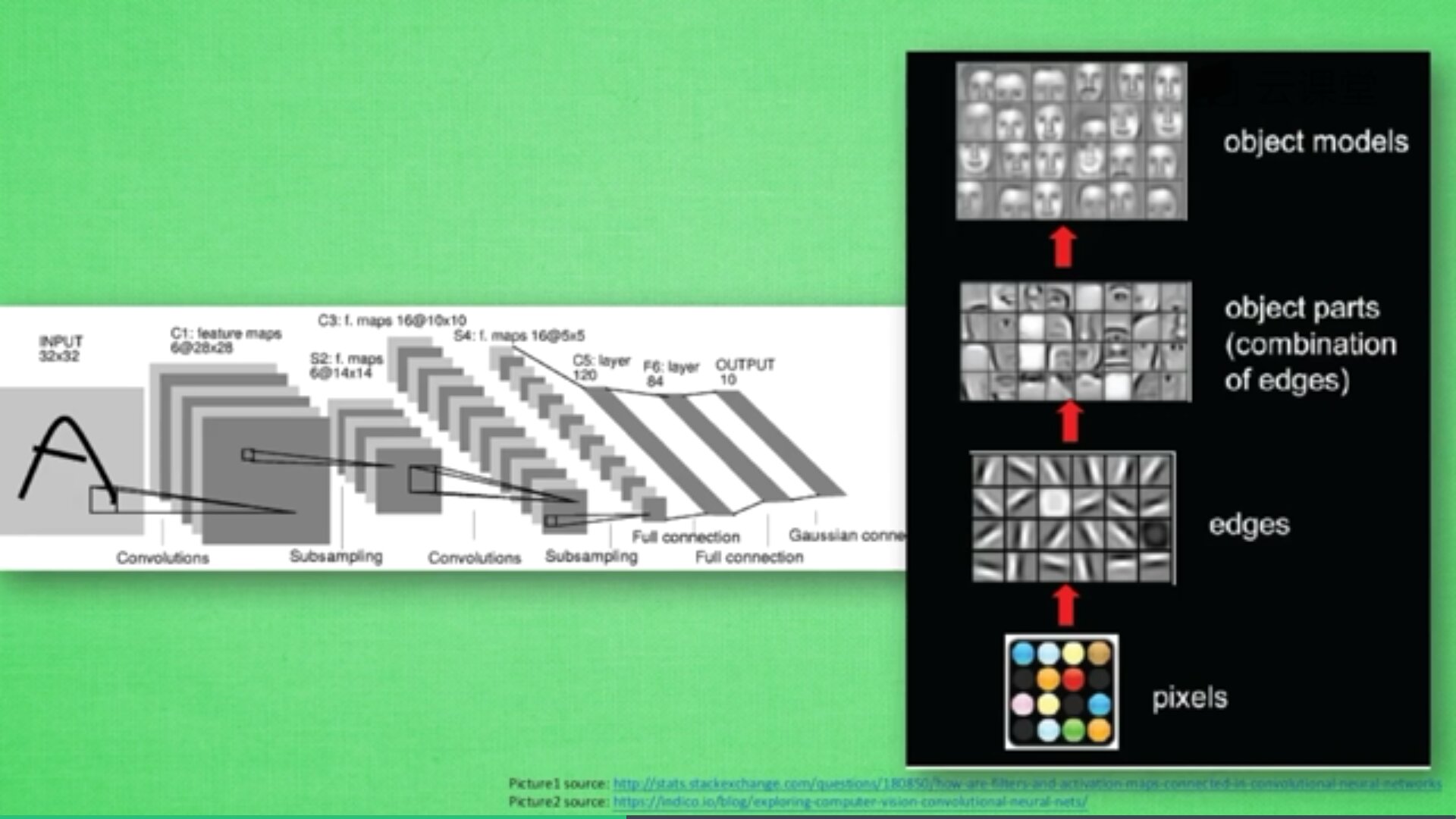
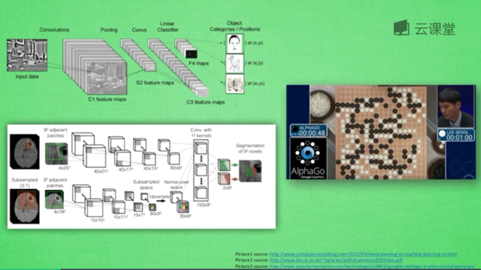
卷积神经网络批量过滤器,持续不断在图片上滚动搜集信息,每一次搜索都是一小块信息,整理这一小块信息之后得到边缘信息。比如第一次得出眼睛鼻子轮廓等,再经过一次过滤,将脸部信息总结出来,再将这些信息放到全神经网络中进行训练,反复扫描最终得出的分类结果。如下图所示,猫的一张照片需要转换为数学的形式,这里采用长宽高存储,其中黑白照片的高度为1,彩色照片的高度为3(RGB)。

过滤器搜集这些信息,将得到一个更小的图片,再经过压缩增高信息嵌入到普通神经层上,最终得到分类的结果,这个过程即是卷积。Convnets是一种在空间上共享参数的神经网络,如下图所示,它将一张RGB图片进行压缩增高,得到一个很长的结果。

一个卷积网络是组成深度网络的基础,我们将使用数层卷积而不是数层的矩阵相乘。如上图所示,让它形成金字塔形状,金字塔底是一个非常大而浅的图片,仅包括红绿蓝,通过卷积操作逐渐挤压空间的维度,同时不断增加深度,使深度信息基本上可以表示出复杂的语义。同时,你可以在金字塔的顶端实现一个分类器,所有空间信息都被压缩成一个标识,只有把图片映射到不同类的信息保留,这就是CNN的总体思想。
上图的具体流程如下:
- 首先,这是有一张彩色图片,它包括RGB三原色分量,图像的长和宽为256*256,三个层面分别对应红(R)、绿(G)、蓝(B)三个图层,也可以看作像素点的厚度。
- 其次,CNN将图片的长度和宽度进行压缩,变成128x128x16的方块,压缩的方法是把图片的长度和宽度压小,从而增高厚度。
- 再次,继续压缩至64x64x64,直至32x32x256,此时它变成了一个很厚的长条方块,我们这里称之为分类器Classifier。该分类器能够将我们的分类结果进行预测,MNIST手写体数据集预测结果是10个数字,比如[0,0,0,1,0,0,0,0,0,0]表示预测的结果是数字3,Classifier在这里就相当于这10个序列。
- 最后,CNN通过不断压缩图片的长度和宽度,增加厚度,最终会变成了一个很厚的分类器,从而进行分类预测。
近几年神经网络飞速发展,其中一个很重要的原因就是CNN卷积神经网络的提出,这也是计算机视觉处理的飞跃提升。关于TensorFlow中的CNN,Google公司也出了一个非常精彩的视频教程,也推荐大家去学习。
2.模型设计
该部分采用Keras搭建四层CNN网络,是本文的核心过程,再次感谢刘兄代码,受益匪浅。
#----------------------------------------------------------------
#                         第六步 CNN模型设计
#----------------------------------------------------------------
from keras.models import Sequential
from keras.layers import Conv2D, MaxPooling2D, GlobalAveragePooling2D, BatchNormalization, Dropout, Dense

#定义模型
def create_model(optimizer='adam', kernel_initializer='he_normal', activation='relu'):
    #第一个卷积层
    model = Sequential()
    model.add(Conv2D(filters=16, kernel_size=3, padding='same', input_shape=(32, 32, 1), kernel_initializer=kernel_initializer, activation=activation))
    model.add(BatchNormalization())
    model.add(MaxPooling2D(pool_size=2))
    model.add(Dropout(0.2))

    #第二个卷积层
    model.add(Conv2D(filters=32, kernel_size=3, padding='same', kernel_initializer=kernel_initializer, activation=activation))
    model.add(BatchNormalization())
    model.add(MaxPooling2D(pool_size=2))
    model.add(Dropout(0.2))

    #第三个卷积层
    model.add(Conv2D(filters=64, kernel_size=3, padding='same', kernel_initializer=kernel_initializer, activation=activation))
    model.add(BatchNormalization())
    model.add(MaxPooling2D(pool_size=2))
    model.add(Dropout(0.2))

    #第四个卷积层
    model.add(Conv2D(filters=128, kernel_size=3, padding='same', kernel_initializer=kernel_initializer, activation=activation))
    model.add(BatchNormalization())
    model.add(MaxPooling2D(pool_size=2))
    model.add(Dropout(0.2))
    model.add(GlobalAveragePooling2D())

    #全连接层输出28类结果
    model.add(Dense(28, activation='softmax'))

    #损失函数定义
    model.compile(loss='categorical_crossentropy', metrics=['accuracy'], optimizer=optimizer)
    return model

#创建模型
model = create_model(optimizer='Adam', kernel_initializer='uniform', activation='relu')
model.summary()
模型包括四个卷积神经网络,再通过全连接层实现分类。每个卷积层内容如下:
- 输入层包括16个特征图,大小为3×3和一个relu激活函数;
- 接着是批量标准化层,主要用于解决特征分布在训练和测试数据中的变化,BN层添加在激活函数前,对输入激活函数的输入进行归一化,解决数据发送偏移和增大的影响;
- 池化层主要对输入进行下采样,从而减小参数的学习次数和训练时间;
- 使用dropout正则化,设置参数为0.2,即被配置为随机排除层中20%的神经元以减少过度拟合。
总共是16、32、64、128个元素的隐藏层,最后通过输出层(类别28),并使用softmax激活函数,利用交叉熵作为损失函数。整个模型的结构输出如下所示:
Model: "sequential_1"
_________________________________________________________________
Layer (type)                 Output Shape              Param #
=================================================================
conv2d_1 (Conv2D)            (None, 32, 32, 16)        160
_________________________________________________________________
batch_normalization_1 (Batch (None, 32, 32, 16)        64
_________________________________________________________________
max_pooling2d_1 (MaxPooling2 (None, 16, 16, 16)        0
_________________________________________________________________
dropout_1 (Dropout)          (None, 16, 16, 16)        0
_________________________________________________________________
conv2d_2 (Conv2D)            (None, 16, 16, 32)        4640
_________________________________________________________________
batch_normalization_2 (Batch (None, 16, 16, 32)        128
_________________________________________________________________
max_pooling2d_2 (MaxPooling2 (None, 8, 8, 32)          0
_________________________________________________________________
dropout_2 (Dropout)          (None, 8, 8, 32)          0
_________________________________________________________________
conv2d_3 (Conv2D)            (None, 8, 8, 64)          18496
_________________________________________________________________
batch_normalization_3 (Batch (None, 8, 8, 64)          256
_________________________________________________________________
max_pooling2d_3 (MaxPooling2 (None, 4, 4, 64)          0
_________________________________________________________________
dropout_3 (Dropout)          (None, 4, 4, 64)          0
_________________________________________________________________
conv2d_4 (Conv2D)            (None, 4, 4, 128)         73856
_________________________________________________________________
batch_normalization_4 (Batch (None, 4, 4, 128)         512
_________________________________________________________________
max_pooling2d_4 (MaxPooling2 (None, 2, 2, 128)         0
_________________________________________________________________
dropout_4 (Dropout)          (None, 2, 2, 128)         0
_________________________________________________________________
global_average_pooling2d_1 ( (None, 128)               0
_________________________________________________________________
dense_1 (Dense)              (None, 28)                3612
=================================================================
Total params: 101,724
Trainable params: 101,244
Non-trainable params: 480
_________________________________________________________________
3.模型绘制
在Keras中,我们可以调用 keras.utils.vis_utils 模块绘制模型,该模块提供了graphviz绘制功能。
#----------------------------------------------------------------
#                         第七步 模型绘制
#----------------------------------------------------------------
from keras.utils.vis_utils import plot_model
from IPython.display import Image as IPythonImage

plot_model(model, to_file="model.png", show_shapes=True)
display(IPythonImage('model.png'))
输出结果如下图所示:

graphviz报错解决
AssertionError: “dot” with args [’-Tps’, ‘C:\Users\…\AppData\Local\Temp\tmp8tx_96_r’] returned code: 1,这是由于pydot已经停止开发了,在Python3.5和Python3.6中无法所用。解决方案:
- 第一步,打开Anaconda的命令行,并卸载pydot扩展包:pip uninstall pydot
- 第二步,安装pydotplus扩展包:pip install pydotplus,如果报错反复卸载安装 o(╥﹏╥)o
pip install --target=“c:\software\program software\anaconda3\envs\tensorflow\lib\site-packages” pydotplus- 第三步,找到keras里面的utils.vis_utils.py,把pydot的都替换成pydotplus
import pydotplus as pydot
- 下载地址:https://graphviz.gitlab.io/_pages/Download/windows/graphviz-2.38.msi
- pydot用法:https://blog.csdn.net/lizzy05/article/details/88529483
- 解决方法:https://blog.csdn.net/qq_27825451/article/details/89338222


五.实验评估
1.模型训练
接着是模型训练,这里使用检查点来保存模型权重,同时batch大小设置为20,epochs设置为15。
#----------------------------------------------------------------
#                         第八步 模型训练
#----------------------------------------------------------------
from keras.callbacks import ModelCheckpoint
checkpointer = ModelCheckpoint(filepath='weights.hdf5',
                               verbose=1,
                               save_best_only=True)
history = model.fit(training_letters_images_scaled,
                    training_letters_labels_encoded,
                    validation_data=(testing_letters_images_scaled,
                                     testing_letters_labels_encoded),
                    epochs=15,
                    batch_size=20,
                    verbose=1,
                    callbacks=[checkpointer])
print(history)
训练过程如下图所示:
Train on 13440 samples, validate on 3360 samples
Epoch 1/15
13440/13440 [==============================] - 21s 2ms/step - loss: 1.3694 - accuracy: 0.5759 - val_loss: 0.8664 - val_accuracy: 0.7271

Epoch 00001: val_loss improved from inf to 0.86641, saving model to weights.hdf5
Epoch 2/15
13440/13440 [==============================] - 20s 1ms/step - loss: 0.4939 - accuracy: 0.8394 - val_loss: 0.2832 - val_accuracy: 0.9125

Epoch 00002: val_loss improved from 0.86641 to 0.28324, saving model to weights.hdf5
Epoch 3/15
13440/13440 [==============================] - 20s 1ms/step - loss: 0.3559 - accuracy: 0.8861 - val_loss: 0.4726 - val_accuracy: 0.8438

Epoch 00003: val_loss did not improve from 0.28324
Epoch 4/15
13440/13440 [==============================] - 20s 1ms/step - loss: 0.2913 - accuracy: 0.9059 - val_loss: 0.2211 - val_accuracy: 0.9292

Epoch 00004: val_loss improved from 0.28324 to 0.22108, saving model to weights.hdf5
Epoch 5/15
13440/13440 [==============================] - 21s 2ms/step - loss: 0.2557 - accuracy: 0.9183 - val_loss: 0.1782 - val_accuracy: 0.9429

Epoch 00005: val_loss improved from 0.22108 to 0.17819, saving model to weights.hdf5
Epoch 6/15
13440/13440 [==============================] - 18s 1ms/step - loss: 0.2287 - accuracy: 0.9237 - val_loss: 0.1602 - val_accuracy: 0.9518

Epoch 00006: val_loss improved from 0.17819 to 0.16022, saving model to weights.hdf5
Epoch 7/15
13440/13440 [==============================] - 21s 2ms/step - loss: 0.2162 - accuracy: 0.9295 - val_loss: 0.1964 - val_accuracy: 0.9417

Epoch 00007: val_loss did not improve from 0.16022
Epoch 8/15
13440/13440 [==============================] - 20s 1ms/step - loss: 0.1913 - accuracy: 0.9365 - val_loss: 0.1751 - val_accuracy: 0.9491

Epoch 00008: val_loss did not improve from 0.16022
Epoch 9/15
13440/13440 [==============================] - 18s 1ms/step - loss: 0.1791 - accuracy: 0.9412 - val_loss: 0.1389 - val_accuracy: 0.9640

Epoch 00009: val_loss improved from 0.16022 to 0.13888, saving model to weights.hdf5
Epoch 10/15
13440/13440 [==============================] - 19s 1ms/step - loss: 0.1651 - accuracy: 0.9434 - val_loss: 0.1581 - val_accuracy: 0.9533

Epoch 00010: val_loss did not improve from 0.13888
Epoch 11/15
13440/13440 [==============================] - 19s 1ms/step - loss: 0.1705 - accuracy: 0.9426 - val_loss: 0.2523 - val_accuracy: 0.9140

Epoch 00011: val_loss did not improve from 0.13888
Epoch 12/15
13440/13440 [==============================] - 19s 1ms/step - loss: 0.1648 - accuracy: 0.9455 - val_loss: 0.3119 - val_accuracy: 0.9071

Epoch 00012: val_loss did not improve from 0.13888
Epoch 13/15
13440/13440 [==============================] - 21s 2ms/step - loss: 0.1517 - accuracy: 0.9503 - val_loss: 0.1698 - val_accuracy: 0.9497

Epoch 00013: val_loss did not improve from 0.13888
Epoch 14/15
13440/13440 [==============================] - 18s 1ms/step - loss: 0.1429 - accuracy: 0.9529 - val_loss: 0.1674 - val_accuracy: 0.9539

Epoch 00014: val_loss did not improve from 0.13888
Epoch 15/15
13440/13440 [==============================] - 19s 1ms/step - loss: 0.1363 - accuracy: 0.9527 - val_loss: 0.1502 - val_accuracy: 0.9598

Epoch 00015: val_loss did not improve from 0.13888
<keras.callbacks.callbacks.History object at 0x000001EF27F6DDA0>
2.绘制误差和准确率曲线
该部分核心代码如下:
#----------------------------------------------------------------
# 第九步 绘制图形
#----------------------------------------------------------------
import matplotlib.pyplot as plt
def plot_loss_accuracy(history):
# Loss
plt.figure(figsize=[8,6])
plt.plot(history.history['loss'],'r',linewidth=3.0)
plt.plot(history.history['val_loss'],'b',linewidth=3.0)
plt.legend(['Training loss', 'Validation Loss'],fontsize=18)
plt.xlabel('Epochs ',fontsize=16)
plt.ylabel('Loss',fontsize=16)
plt.title('Loss Curves',fontsize=16)
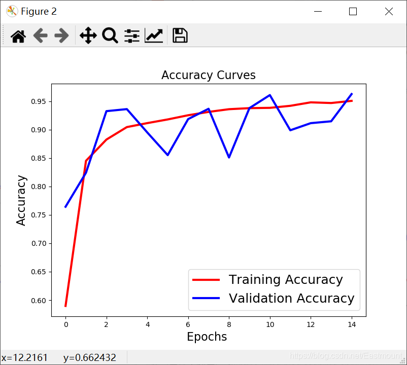
# Accuracy
plt.figure(figsize=[8,6])
plt.plot(history.history['accuracy'],'r',linewidth=3.0)
plt.plot(history.history['val_accuracy'],'b',linewidth=3.0)
plt.legend(['Training Accuracy', 'Validation Accuracy'],fontsize=18)
plt.xlabel('Epochs ',fontsize=16)
plt.ylabel('Accuracy',fontsize=16)
plt.title('Accuracy Curves',fontsize=16)
plot_loss_accuracy(history)
绘制如下图所示结果。

3.模型评估
注意,由于上一个步骤已经训练好了模型,这里我们增加一个判断,防止重复训练,直接调用weights.hdf5模型进行预测。
#----------------------------------------------------------------
#                         第八步 模型训练+输出结果
#----------------------------------------------------------------
from keras.callbacks import ModelCheckpoint
from sklearn.metrics import classification_report
import matplotlib.pyplot as plt

#绘制图形
def plot_loss_accuracy(history):
    # Loss
    plt.figure(figsize=[8,6])
    plt.plot(history.history['loss'],'r',linewidth=3.0)
    plt.plot(history.history['val_loss'],'b',linewidth=3.0)
    plt.legend(['Training loss', 'Validation Loss'],fontsize=18)
    plt.xlabel('Epochs ',fontsize=16)
    plt.ylabel('Loss',fontsize=16)
    plt.title('Loss Curves',fontsize=16)

    # Accuracy
    plt.figure(figsize=[8,6])
    plt.plot(history.history['accuracy'],'r',linewidth=3.0)
    plt.plot(history.history['val_accuracy'],'b',linewidth=3.0)
    plt.legend(['Training Accuracy', 'Validation Accuracy'],fontsize=18)
    plt.xlabel('Epochs ',fontsize=16)
    plt.ylabel('Accuracy',fontsize=16)
    plt.title('Accuracy Curves',fontsize=16)

#混淆矩阵
def get_predicted_classes(model, data, labels=None):
    image_predictions = model.predict(data)
    predicted_classes = np.argmax(image_predictions, axis=1)
    true_classes = np.argmax(labels, axis=1)
    return predicted_classes, true_classes, image_predictions

def get_classification_report(y_true, y_pred):
    print(classification_report(y_true, y_pred, digits=4)) #小数点4位

checkpointer = ModelCheckpoint(filepath='weights.hdf5',
                               verbose=1,
                               save_best_only=True)
flag = "test"
if flag=="train":
    history = model.fit(training_letters_images_scaled,
                        training_letters_labels_encoded,
                        validation_data=(testing_letters_images_scaled,
                                         testing_letters_labels_encoded),
                        epochs=15,
                        batch_size=20,
                        verbose=1,
                        callbacks=[checkpointer])
    print(history)
    plot_loss_accuracy(history)
else:
    #加载具有最佳验证损失的模型
    model.load_weights('weights.hdf5')
    metrics = model.evaluate(testing_letters_images_scaled,
                             testing_letters_labels_encoded,
                             verbose=1)
    print("Test Accuracy: {}".format(metrics[1]))
    print("Test Loss: {}".format(metrics[0]))

    y_pred, y_true, image_predictions = get_predicted_classes(model,
                                                              testing_letters_images_scaled,
                                                              testing_letters_labels_encoded)
    get_classification_report(y_true, y_pred)
最终输出结果如下所示:
3360/3360 [==============================] - 2s 466us/step
Test Accuracy: 0.9639880657196045
Test Loss: 0.13888128581900328
              precision    recall  f1-score   support

           0     0.9756    1.0000    0.9877       120
           1     0.9675    0.9917    0.9794       120
           2     0.9187    0.9417    0.9300       120
           3     0.9504    0.9583    0.9544       120
           4     0.9600    1.0000    0.9796       120
           5     0.9590    0.9750    0.9669       120
           6     0.9587    0.9667    0.9627       120
           7     0.9435    0.9750    0.9590       120
           8     0.9134    0.9667    0.9393       120
           9     0.9370    0.9917    0.9636       120
          10     0.9817    0.8917    0.9345       120
          11     0.9008    0.9833    0.9402       120
          12     0.9832    0.9750    0.9791       120
          13     0.9818    0.9000    0.9391       120
          14     0.9912    0.9333    0.9614       120
          15     0.9375    1.0000    0.9677       120
          16     0.9912    0.9417    0.9658       120
          17     0.9912    0.9417    0.9658       120
          18     0.9914    0.9583    0.9746       120
          19     0.9286    0.9750    0.9512       120
          20     0.9739    0.9333    0.9532       120
          21     0.9600    1.0000    0.9796       120
          22     1.0000    1.0000    1.0000       120
          23     0.9916    0.9833    0.9874       120
          24     0.9737    0.9250    0.9487       120
          25     0.9832    0.9750    0.9791       120
          26     0.9741    0.9417    0.9576       120
          27     1.0000    0.9667    0.9831       120

    accuracy                         0.9640      3360
   macro avg     0.9650    0.9640    0.9640      3360
weighted avg     0.9650    0.9640    0.9640      3360
4.绘制预测图片
#----------------------------------------------------------------
#                         第九步 绘制测试图像
#----------------------------------------------------------------
fig = plt.figure(0, figsize=(14,14))
indices = np.random.randint(0, testing_letters_labels.shape[0], size=49)
y_pred = np.argmax(model.predict(training_letters_images_scaled), axis=1)

for i, idx in enumerate(indices):
    plt.subplot(7,7,i+1)

    image_array = training_letters_images_scaled[idx][:,:,0]
    image_array = np.flip(image_array, 0)
    image_array = rotate(image_array, -90)

    plt.imshow(image_array, cmap='gray')
    plt.title("Pred: {} - Label: {}".format(y_pred[idx],
              (training_letters_labels[idx] -1)))
    plt.xticks([])
    plt.yticks([])
plt.show()
plt.savefig("resutl.png")
输出结果如下图所示:

六.完整代码
最终代码如下:
# -*- coding: utf-8 -*-
"""
Created on Wed Jul  7 18:54:36 2021
@author: xiuzhang CSDN
参考:刘润森老师博客 推荐大家关注 很厉害的一位CV大佬
     https://maoli.blog.csdn.net/article/details/117688738
"""
import numpy as np
import pandas as pd
from IPython.display import display
import csv
from PIL import Image
from scipy.ndimage import rotate

#----------------------------------------------------------------
#                      第一步 读取数据
#----------------------------------------------------------------
#训练数据images和labels
letters_training_images_file_path = "dataset/csvTrainImages 13440x1024.csv"
letters_training_labels_file_path = "dataset/csvTrainLabel 13440x1.csv"
#测试数据images和labels
letters_testing_images_file_path = "dataset/csvTestImages 3360x1024.csv"
letters_testing_labels_file_path = "dataset/csvTestLabel 3360x1.csv"

#加载数据
training_letters_images = pd.read_csv(letters_training_images_file_path, header=None)
training_letters_labels = pd.read_csv(letters_training_labels_file_path, header=None)
testing_letters_images = pd.read_csv(letters_testing_images_file_path, header=None)
testing_letters_labels = pd.read_csv(letters_testing_labels_file_path, header=None)
print("%d个32x32像素的训练阿拉伯字母图像" % training_letters_images.shape[0])
print("%d个32x32像素的测试阿拉伯字母图像" % testing_letters_images.shape[0])
print(training_letters_images.head())
print(np.unique(training_letters_labels))


#----------------------------------------------------------------
#                      第二步 数值转换为图像特征
#----------------------------------------------------------------
#原始数据集被反射使用np.flip翻转它 通过rotate旋转从而获得更好的图像
def convert_values_to_image(image_values, display=False):
    #转换成32x32
    image_array = np.asarray(image_values)
    image_array = image_array.reshape(32,32).astype('uint8')
    #翻转+旋转
    image_array = np.flip(image_array, 0)
    image_array = rotate(image_array, -90)
    #图像显示
    new_image = Image.fromarray(image_array)
    if display == True:
        new_image.show()
    return new_image

convert_values_to_image(training_letters_images.loc[0], True)


#----------------------------------------------------------------
#                      第三步 图像标准化处理
#----------------------------------------------------------------
training_letters_images_scaled = training_letters_images.values.astype('float32')/255
training_letters_labels = training_letters_labels.values.astype('int32')
testing_letters_images_scaled = testing_letters_images.values.astype('float32')/255
testing_letters_labels = testing_letters_labels.values.astype('int32')
print("Training images of letters after scaling")
print(training_letters_images_scaled.shape)
print(training_letters_images_scaled[0:5])


#----------------------------------------------------------------
#                      第四步 输出One-hot编码转换
#----------------------------------------------------------------
import keras
from keras.utils import to_categorical
number_of_classes = 28
training_letters_labels_encoded = to_categorical(training_letters_labels-1,
                                                 num_classes=number_of_classes)
testing_letters_labels_encoded = to_categorical(testing_letters_labels-1,
                                                num_classes=number_of_classes)
print(training_letters_labels)
print(training_letters_labels_encoded)
print(training_letters_images_scaled.shape)
# (13440, 1024)


#----------------------------------------------------------------
#                         第五步 形状修改
#----------------------------------------------------------------
#输入形状 32x32x1
training_letters_images_scaled = training_letters_images_scaled.reshape([-1, 32, 32, 1])
testing_letters_images_scaled = testing_letters_images_scaled.reshape([-1, 32, 32, 1])
print(training_letters_images_scaled.shape,
      training_letters_labels_encoded.shape,
      testing_letters_images_scaled.shape,
      testing_letters_labels_encoded.shape)
# (13440, 32, 32, 1) (13440, 28) (3360, 32, 32, 1) (3360, 28)


#----------------------------------------------------------------
#                         第六步 CNN模型设计
#----------------------------------------------------------------
from keras.models import Sequential
from keras.layers import Conv2D, MaxPooling2D, GlobalAveragePooling2D, BatchNormalization, Dropout, Dense

#定义模型
def create_model(optimizer='adam', kernel_initializer='he_normal', activation='relu'):
    #第一个卷积层
    model = Sequential()
    model.add(Conv2D(filters=16, kernel_size=3, padding='same', input_shape=(32, 32, 1), kernel_initializer=kernel_initializer, activation=activation))
    model.add(BatchNormalization())
    model.add(MaxPooling2D(pool_size=2))
    model.add(Dropout(0.2))

    #第二个卷积层
    model.add(Conv2D(filters=32, kernel_size=3, padding='same', kernel_initializer=kernel_initializer, activation=activation))
    model.add(BatchNormalization())
    model.add(MaxPooling2D(pool_size=2))
    model.add(Dropout(0.2))

    #第三个卷积层
    model.add(Conv2D(filters=64, kernel_size=3, padding='same', kernel_initializer=kernel_initializer, activation=activation))
    model.add(BatchNormalization())
    model.add(MaxPooling2D(pool_size=2))
    model.add(Dropout(0.2))

    #第四个卷积层
    model.add(Conv2D(filters=128, kernel_size=3, padding='same', kernel_initializer=kernel_initializer, activation=activation))
    model.add(BatchNormalization())
    model.add(MaxPooling2D(pool_size=2))
    model.add(Dropout(0.2))
    model.add(GlobalAveragePooling2D())

    #全连接层输出28类结果
    model.add(Dense(28, activation='softmax'))

    #损失函数定义
    model.compile(loss='categorical_crossentropy', metrics=['accuracy'], optimizer=optimizer)
    return model

#创建模型
model = create_model(optimizer='Adam', kernel_initializer='uniform', activation='relu')
model.summary()


#----------------------------------------------------------------
#                         第七步 模型绘制
#----------------------------------------------------------------
from keras.utils.vis_utils import plot_model
from IPython.display import Image as IPythonImage

plot_model(model, to_file="model.png", show_shapes=True)
display(IPythonImage('model.png'))


#----------------------------------------------------------------
#                         第八步 模型训练+输出结果
#----------------------------------------------------------------
from keras.callbacks import ModelCheckpoint
from sklearn.metrics import classification_report
import matplotlib.pyplot as plt

#绘制图形
def plot_loss_accuracy(history):
    # Loss
    plt.figure(figsize=[8,6])
    plt.plot(history.history['loss'],'r',linewidth=3.0)
    plt.plot(history.history['val_loss'],'b',linewidth=3.0)
    plt.legend(['Training loss', 'Validation Loss'],fontsize=18)
    plt.xlabel('Epochs ',fontsize=16)
    plt.ylabel('Loss',fontsize=16)
    plt.title('Loss Curves',fontsize=16)

    # Accuracy
    plt.figure(figsize=[8,6])
    plt.plot(history.history['accuracy'],'r',linewidth=3.0)
    plt.plot(history.history['val_accuracy'],'b',linewidth=3.0)
    plt.legend(['Training Accuracy', 'Validation Accuracy'],fontsize=18)
    plt.xlabel('Epochs ',fontsize=16)
    plt.ylabel('Accuracy',fontsize=16)
    plt.title('Accuracy Curves',fontsize=16)

#混淆矩阵
def get_predicted_classes(model, data, labels=None):
    image_predictions = model.predict(data)
    predicted_classes = np.argmax(image_predictions, axis=1)
    true_classes = np.argmax(labels, axis=1)
    return predicted_classes, true_classes, image_predictions

def get_classification_report(y_true, y_pred):
    print(classification_report(y_true, y_pred, digits=4)) #小数点4位

checkpointer = ModelCheckpoint(filepath='weights.hdf5',
                               verbose=1,
                               save_best_only=True)
flag = "test"
if flag=="train":
    history = model.fit(training_letters_images_scaled,
                        training_letters_labels_encoded,
                        validation_data=(testing_letters_images_scaled,
                                         testing_letters_labels_encoded),
                        epochs=15,
                        batch_size=20,
                        verbose=1,
                        callbacks=[checkpointer])
    print(history)
    plot_loss_accuracy(history)
else:
    #加载具有最佳验证损失的模型
    model.load_weights('weights.hdf5')
    metrics = model.evaluate(testing_letters_images_scaled,
                             testing_letters_labels_encoded,
                             verbose=1)
    print("Test Accuracy: {}".format(metrics[1]))
    print("Test Loss: {}".format(metrics[0]))

    y_pred, y_true, image_predictions = get_predicted_classes(model,
                                                              testing_letters_images_scaled,
                                                              testing_letters_labels_encoded)
    get_classification_report(y_true, y_pred)

	#----------------------------------------------------------------
	#                         第九步 绘制测试图像
	#----------------------------------------------------------------
	fig = plt.figure(0, figsize=(14,14))
	indices = np.random.randint(0, testing_letters_labels.shape[0], size=49)
	y_pred = np.argmax(model.predict(training_letters_images_scaled), axis=1)

	for i, idx in enumerate(indices):
	    plt.subplot(7,7,i+1)

	    image_array = training_letters_images_scaled[idx][:,:,0]
	    image_array = np.flip(image_array, 0)
	    image_array = rotate(image_array, -90)

	    plt.imshow(image_array, cmap='gray')
	    plt.title("Pred: {} - Label: {}".format(y_pred[idx],
	              (training_letters_labels[idx] -1)))
	    plt.xticks([])
	    plt.yticks([])
	plt.show()
	plt.savefig("resutl.png")
七.总结
写到这里,这篇文章就介绍结束了,希望对您有所帮助。当然还可以增加热度图以及不同算法的对比,后面尝试分享更前沿的图像分类算法。
- 一.数据集描述
- 二.数据读取
- 三.数据预处理
1.数值特征转换图像
2.图像标准化处理
3.输出One-hot编码转换
4.形状修改 - 四.CNN模型搭建
1.卷积神经网络概念
2.模型设计
3.模型绘制 - 五.实验评估
1.模型训练
2.绘制误差和准确率曲线
3.模型评估
4.绘制预测图片 - 六.完整代码
import seaborn as sns
from sklearn import metrics

Labname = [1,2,3,4,5,6,7,8,9,10,11,12,13,14,
           15,16,17,18,19,20,21,22,23,24,25,26,27,28]
print(y_pre_test)
y_pre_test = [num+1 for num in y_pre_test]
print(np.argmax(testing_letters_labels,axis=1))
confm = metrics.confusion_matrix(testing_letters_labels,
                                 y_pre_test)
plt.figure(figsize=(10,10))
sns.heatmap(confm.T, square=True, annot=True,
            fmt='d', cbar=True, linewidths=.6,
            cmap="YlGnBu")
plt.xlabel('True label',size = 12)
plt.ylabel('Predicted label', size = 12)
plt.xticks(np.arange(28)+0.5, Labname, size = 10)
plt.yticks(np.arange(28)+0.5, Labname, size = 10)
plt.savefig('headmap.png')
plt.show()

真心希望这篇文章对您有所帮助,加油~
- https://github.com/eastmountyxz/AI-for-Keras
- https://github.com/eastmountyxz/AI-for-TensorFlow
(By:Eastmount 2021-10-03 夜于盘州 http://blog.csdn.net/eastmount/ )