文章目录
- 滤波算法
- 准备
- Sobel算子
- 锐化算子
- 高斯滤波算子
- 均值滤波
- 中值滤波
- 最优梯度幅值边缘检测算法
- 图像二值化方法
- 全局迭代法
- 大津法
- 获取图像中的轮廓,对图像中的目标进行计数
- 参考blog
滤波算法
cv.filter2D()
这个就是我们用来滤波的函数,作用大概就是根据传入的图片和kernel来对图片进行卷积
参数:
src: 原图像ddepth: 目标图像深度(指数据类型)kernel: 卷积核anchor: 卷积锚点delta: 偏移量,卷积结果要加上这个数字borderType: 边缘类型
卷积函数(目前只能处理单通道图片)
(now:这个函数实现的不好,滤波效果很差,不用了)
def imgConvolve(image, kernel):
    '''
    :param image: 图片矩阵
    :param kernel: 滤波窗口
    :return:卷积后的矩阵
    '''
    img_h = int(image.shape[0])
    img_w = int(image.shape[1])
    kernel_h = int(kernel.shape[0])
    kernel_w = int(kernel.shape[1])
    # padding
    padding_h = int((kernel_h - 1) / 2)
    padding_w = int((kernel_w - 1) / 2)

    convolve_h = int(img_h + 2 * padding_h)
    convolve_W = int(img_w + 2 * padding_w)

    # 分配空间
    img_padding = np.zeros((convolve_h, convolve_W))
    # 中心填充图片
    img_padding[padding_h:padding_h + img_h, padding_w:padding_w + img_w] = image[:, :]
    # 卷积结果
    image_convolve = np.zeros(image.shape)
    # 卷积
    for i in range(padding_h, padding_h + img_h):
        for j in range(padding_w, padding_w + img_w):
            image_convolve[i - padding_h][j - padding_w] = int(
                np.sum(img_padding[i - padding_h:i + padding_h+1, j - padding_w:j + padding_w+1]*kernel))

    return image_convolve
准备
导入图像
img_bubble=cv.imread('bubble.jpg',0)# 单通道读入
img_rice=cv.imread('rice.png',0)# 单通道读入
bubble:
rice:

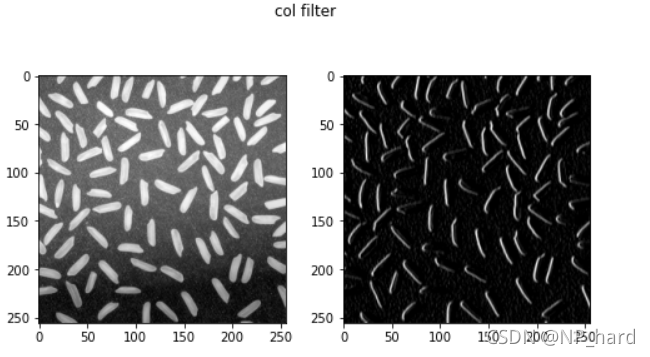
Sobel算子
竖边滤波
可以过滤出图像中竖直方向的边
kernel_col = np.array([[-1,0,1],# 提取竖边的卷积核
                    [-1,0,1],
                    [-1,0,1]])

dst = cv.filter2D(img_rice, -1, kernel_col)

plt.figure(figsize=(8,8)) #设置窗口大小
plt.suptitle('col filter') # 图片名称

plt.subplot(2,2,1)
plt.imshow(img_rice,cmap='gray')
# cv.imshow('rice',img_rice)

plt.subplot(2,2,2)
plt.imshow(dst,cmap='gray')
# cv.imshow('median',dst)
# cv.waitKey(0)
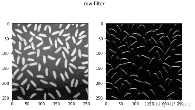
横边滤波
可以过滤出图像中水平方向的边
kernel_row = np.array([[-1,-1,-1],# 提取横边的卷积核
                       [0,0,0],
                       [1,1,1]])

dst = cv.filter2D(img_rice, -1, kernel_row)

plt.figure(figsize=(8,8)) #设置窗口大小
plt.suptitle('row filter') # 图片名称

plt.subplot(2,2,1)
plt.imshow(img_rice,cmap='gray')
# cv.imshow('rice',img_rice)

plt.subplot(2,2,2)
plt.imshow(dst,cmap='gray')
# cv.imshow('median',dst)
# cv.waitKey(0)
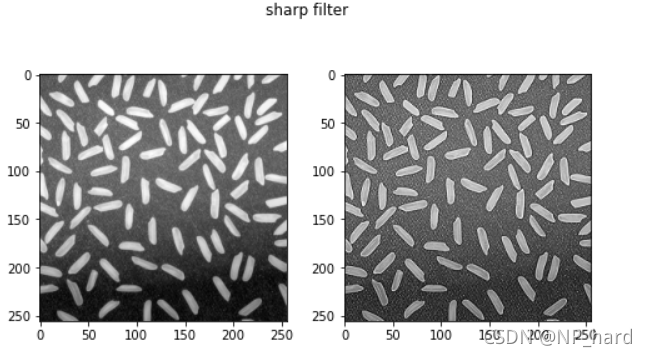
锐化算子
可以将图像进行锐化
kernel_sharp = np.array([[0, -1, 0],
                       [-1, 5, -1],
                       [0, -1, 0]])

dst = cv.filter2D(img_rice, -1, kernel_sharp)

plt.figure(figsize=(8,8)) #设置窗口大小
plt.suptitle('gaussian filter') # 图片名称

plt.subplot(2,2,1)
plt.imshow(img_rice,cmap='gray')
# cv.imshow('rice',img_rice)

plt.subplot(2,2,2)
plt.imshow(dst,cmap='gray')
# cv.imshow('median',dst)
# cv.waitKey(0)
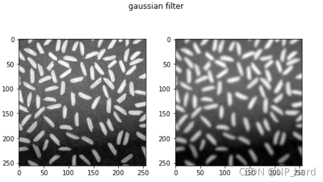
高斯滤波算子
高斯滤波是一种线性平滑滤波,适用于消除高斯噪声,使得图像变得平滑
每一个像素点的值,都由其本身和邻域内的其他像素值经过加权平均后得到
dst = cv.GaussianBlur(img_rice, (11, 11), -1)

plt.figure(figsize=(8,8)) #设置窗口大小
plt.suptitle('gaussian filter') # 图片名称

plt.subplot(2,2,1)
plt.imshow(img_rice,cmap='gray')
# cv.imshow('rice',img_rice)

plt.subplot(2,2,2)
plt.imshow(dst,cmap='gray')
# cv.imshow('median',dst)
# cv.waitKey(0)
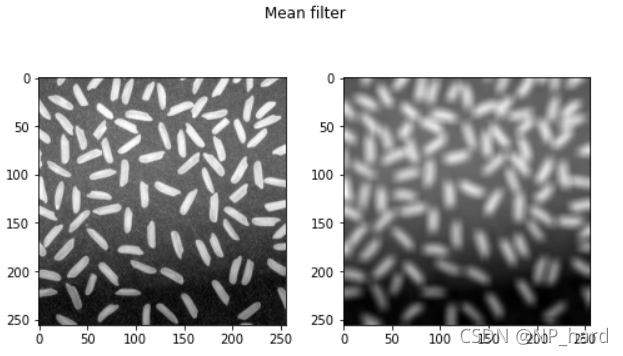
均值滤波
均值滤波是典型的线性滤波算法,每一像素点的灰度值,为该点某邻域窗口内的所有像素点灰度值的平均值
dst = cv.blur(img_rice, (11, 11))

plt.figure(figsize=(8,8)) #设置窗口大小
plt.suptitle('Mean filter') # 图片名称

plt.subplot(2,2,1)
plt.imshow(img_rice,cmap='gray')
# cv.imshow('rice',img_rice)

plt.subplot(2,2,2)
plt.imshow(dst,cmap='gray')
# cv.imshow('median',dst)
# cv.waitKey(0)
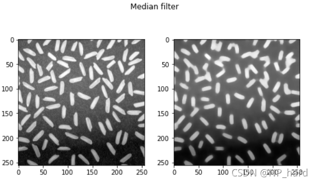
中值滤波
中值滤波法是一种非线性平滑技术,每一像素点的灰度值,为该点某邻域窗口内的所有像素点灰度值的中值
dst = cv.medianBlur(img_rice, 11)

plt.figure(figsize=(8,8)) #设置窗口大小
plt.suptitle('Median filter') # 图片名称

plt.subplot(2,2,1)
plt.imshow(img_rice,cmap='gray')
# cv.imshow('rice',img_rice)

plt.subplot(2,2,2)
plt.imshow(dst,cmap='gray')
# cv.imshow('median',dst)
# cv.waitKey(0)
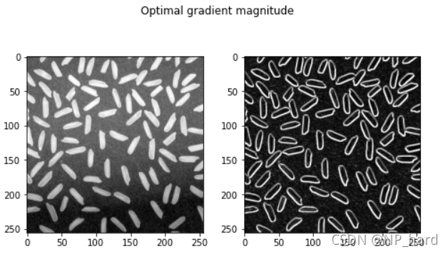
最优梯度幅值边缘检测算法
对米粒图像进行四个方向的滤波,提取出米粒的边缘
这个算法我实现的并不好,运行的可能会比较慢
# cv.imshow('rice',img_rice)
plt.figure(figsize=(8,8)) #设置窗口大小
plt.suptitle('Optimal gradient magnitude') # 图片名称
plt.subplot(2,2,1)
plt.imshow(img_rice,cmap='gray')

kernel_col = np.array([[-1,0,1],# 提取竖边的卷积核
                      [-1,0,1],
                      [-1,0,1]])

kernel_row = np.array([[-1,-1,-1],# 提取横边的卷积核
                       [0,0,0],
                       [1,1,1]])

kernel_incline1 = np.array([[2, 1, 0],# 提取横边的卷积核
                           [1,  0,  -1],
                           [0,  -1,  -2]])
kernel_incline2 = np.array([[0, 1, 2],# 提取横边的卷积核
                           [-1,  0,  1],
                           [-2,  -1,  0]])

dst_1 = cv.filter2D(img_rice, -1, kernel_incline1)
dst_2 = cv.filter2D(img_rice, -1, kernel_incline2)
dst_3 = cv.filter2D(img_rice, -1, kernel_row)
dst_4 = cv.filter2D(img_rice, -1, kernel_col)
dst_tmp1=np.maximum(dst_1,dst_2)
dst_tmp2=np.maximum(dst_3,dst_4)
dst_tmp=np.maximum(dst_tmp1,dst_tmp2)

# cv.imshow('incline_convolve',dst_tmp)
# cv.waitKey(0)
plt.subplot(2,2,2)
plt.imshow(dst_tmp,cmap='gray')
图像二值化方法
全局迭代法
# 计算图像的二值化阈值
def Iteration(img):
    img_array = np.array(img).astype(np.float32)#转化成数组
    I=img_array
    zmax=np.max(I)
    zmin=np.min(I)
    mean=(zmax+zmin)/2#设置初始阈值
    #根据阈值将图像进行分割为前景和背景,分别求出两者的平均灰度  mean_fore和mean_back
    b=1
    m,n=I.shape
    while b==0:
        num_fore=0
        num_back=0
        fnum=0
        bnum=0
        for i in range(1,m):
             for j in range(1,n):
                tmp=I(i,j)
                if tmp>=mean:
                    num_fore+num_fore+1
                    fnum=fnum+int(tmp)  #前景像素的个数以及像素值的总和
                else:
                    num_back=num_back+1
                    bnum=bnum+int(tmp)#背景像素的个数以及像素值的总和
        #计算前景和背景的平均值
        mean_fore=int(fnum/num_fore)
        mean_back=int(bnum/num_back)
        if mean==int((mean_fore+mean_back)/2):
            b=0
        else:
            mean=int((mean_fore+mean_back)/2)
    return mean
# 读取车牌照片
img=cv.imread('car_image/1.JPG')
# 颜色空间转换
img = cv.cvtColor(img,cv.COLOR_BGR2RGB)
gray = cv.cvtColor(img,cv.COLOR_RGB2GRAY)
img = cv.resize(gray,(300,200))#大小
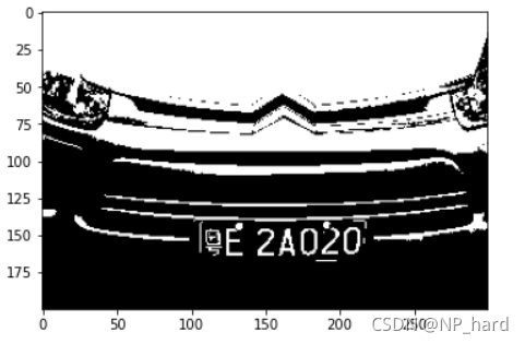
Binar=Iteration(img)
# 二值化
thres, img_binar = cv.threshold(img, Binar, 255, cv.THRESH_BINARY)
print('threshold: ',thres)
plt.imshow(img_binar,cmap=cm.gray)
threshold: 127.0
大津法
def OTSU(img_array):
'''
该函数返回使得类间方差最大的灰度阈值
img_array: 格式为ndarray
'''
height = img_array.shape[0]
width = img_array.shape[1]
count_pixel = np.zeros(256)
# 统计不同灰度值的分布情况
for i in range(height):
for j in range(width):
count_pixel[int(img_array[i][j])] += 1
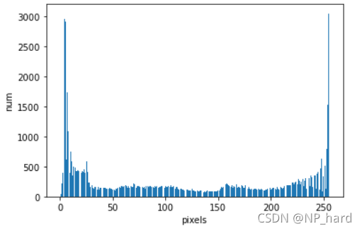
#绘制直方图可以观察像素的分布情况
fig = plt.figure()
ax = fig.add_subplot(111)
ax.bar(np.linspace(0, 255, 256), count_pixel)
ax.set_xlabel("pixels")
ax.set_ylabel("num")
plt.show()
max_variance = 0.0
best_thresold = 0
# 遍历所有灰度值,选择最佳阈值
for thresold in range(256):
n0 = count_pixel[:thresold].sum()# 小于阈值的个数
n1 = count_pixel[thresold:].sum()# 大于阈值的个数
# 属于前景的像素点数占整幅图像的比例
w0 = n0 / (height * width)
# 属于背景的像素点数占整幅图像的比例
w1 = n1 / (height * width)
u0 = 0.0# 前景平均灰度
u1 = 0.0# 背景平均灰度
for i in range(thresold):
u0 += i * count_pixel[i]
for j in range(thresold, 256):
u1 += j * count_pixel[j]
# 图像总平均灰度
u = u0 * w0 + u1 * w1
# 类间方差
tmp_var = w0 * np.power((u - u0), 2) + w1 * np.power((u - u1), 2)
if tmp_var > max_variance:
best_thresold = thresold
max_variance = tmp_var
return best_thresold
# 读取车牌照片
img=cv.imread('car_image/1.JPG')
# 颜色空间转换
img = cv.cvtColor(img,cv.COLOR_BGR2RGB)
gray = cv.cvtColor(img,cv.COLOR_RGB2GRAY)
img = cv.resize(gray,(300,200))#大小
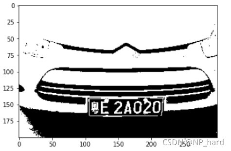
Binar=OTSU(img)
# 二值化
thres, img_binar = cv.threshold(img, Binar, 255, cv.THRESH_BINARY)
print('threshold: ',thres)
plt.imshow(img_binar,cmap=cm.gray)
获取图像中的轮廓,对图像中的目标进行计数
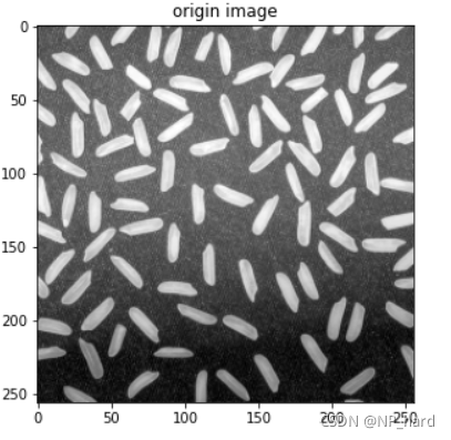
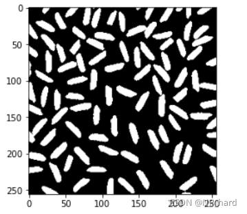
原始图片
plt.figure(figsize=[5,5])
plt.imshow(img_rice,cmap='gray')
plt.title('origin image')
使用局部阈值的大津算法进行图像二值化
dst = cv.adaptiveThreshold(img_rice,255, cv.ADAPTIVE_THRESH_MEAN_C, cv.THRESH_BINARY,101, 1)
element = cv.getStructuringElement(cv.MORPH_CROSS,(3, 3))#形态学去噪
dst=cv.morphologyEx(dst,cv.MORPH_OPEN,element)  #开运算去噪

plt.imshow(dst,cmap='gray')
轮廓检测函数
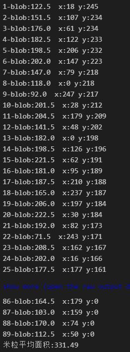
contours, hierarchy = cv.findContours(dst,cv.RETR_EXTERNAL,cv.CHAIN_APPROX_SIMPLE)
cv.drawContours(dst,contours,-1,(120,0,0),2)  #绘制轮廓
count=0 #米粒总数
ares_avrg=0 #米粒平均
img=dst
#遍历找到的所有米粒
for cont in contours:
ares = cv.contourArea(cont)#计算包围性状的面积
if ares<50: #过滤面积小于10的形状
continue
count+=1 #总体计数加1
ares_avrg+=ares
print("{}-blob:{}".format(count,ares),end=" ") #打印出每个米粒的面积
rect = cv.boundingRect(cont) #提取矩形坐标
print("x:{} y:{}".format(rect[0],rect[1]))#打印坐标
cv.rectangle(img,rect,(0xFF, 0xFF, 0xFF),1)#绘制矩形
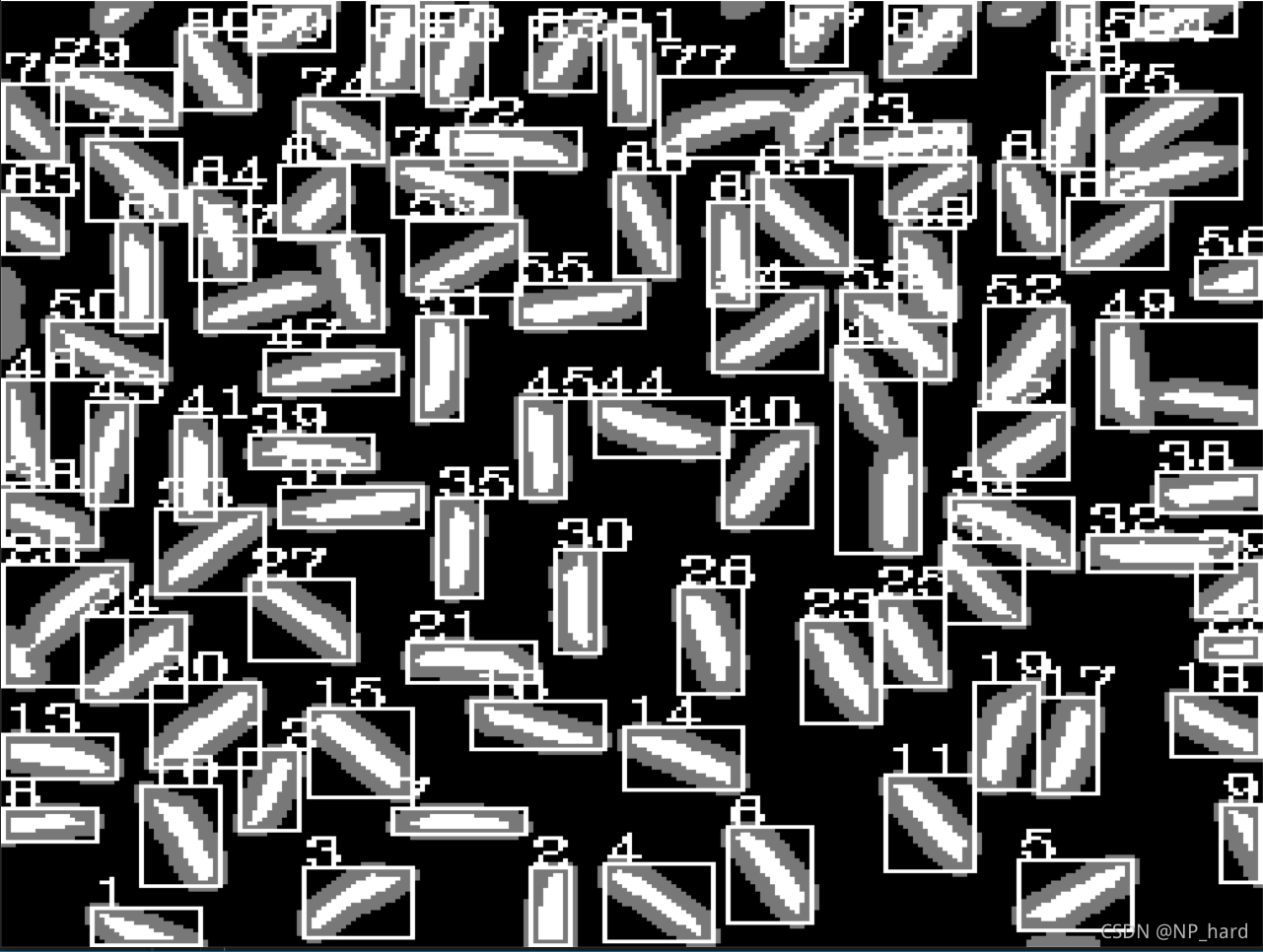
y=10 if rect[1]<10 else rect[1] #防止编号到图片之外
cv.putText(img,str(count), (rect[0], y), cv.FONT_HERSHEY_COMPLEX, 0.4, (255, 160, 180), 1) #在米粒左上角写上编号
print("米粒平均面积:{}".format(round(ares_avrg/ares,2))) #打印出每个米粒的面积
cv.namedWindow("origin", 2) #创建一个窗口
cv.imshow('origin', img_rice) #显示原始图片
cv.namedWindow("dst", 2) #创建一个窗口
cv.imshow("dst", img) #显示灰度图
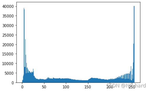
plt.hist(gray.ravel(), 256, [0, 256]) #计算灰度直方图
plt.show()
cv.waitKey(0)
迭代结果
灰度值分布的直方图
对识别出的目标进行标记
参考blog
- blog1
- blog2
- blog3
- blog4