OpenCV-Python实战（4）——OpenCV常见图像处理技术（❤️万字长文，含大量示例❤️）_盼小辉丶的博客

0. 前言

图像处理技术是计算机视觉项目的核心，通常是计算机视觉项目中的关键工具，可以使用它们来完成各种计算机视觉任务。因此，如果要构建计算机视觉项目，就需要对图像处理有足够的了解。在本文中，将介绍计算机视觉项目中常见的图像处理技术，主要包括图像的几何变换和图像滤波等。

1. 拆分与合并通道

再进行图像处理时，有时我们仅需要使用特定通道。因此，必须首先将多通道图像拆分为多个单通道图像，为了拆分通道，可以使用 cv2.split() 函数，cv2.split() 函数将源多通道图像拆分为多个单通道图像。此外，处理完成后，可能希望将多个的单通道图像合并创建为一个多通道图像，为了合并通道，可以使用 cv2.merge() 函数，cv2.merge() 函数将多个单通道图像合并为一个多通道图像。
使用 cv2.split() 函数，从加载的 BGR 图像中获取三个通道：

# 通道拆分
image = cv2.imread('sigonghuiye.jpeg')
(b, g, r) = cv2.split(image)

使用 cv2.merge() 函数，将三个通道合并构建 BGR 图像：

# 通道合并
image_copy = cv2.merge((b, g, r))

需要注意的是，cv2.split() 是一个耗时的操作，所以应该只在绝对必要的时候使用它。作为替代，可以使用 NumPy 切片语法来处理特定通道。例如，如果要获取图像的蓝色通道：

b = image[:, :, 0]

此外，可以消除多通道图像的某些通道(通过将通道值设置为 0 )，得到的图像具有相同数量的通道，但相应通道中的值为 0；例如，如果要消除 BGR 图像的蓝色通道：

image_without_blue = image.copy()
image_without_blue[:, :, 0] = 0

消除其他通道的方法与上述代码原理相同：

# 红蓝通道
image_without_green = image.copy()
image_without_green[:,:,1] = 0
# 蓝绿通道
image_without_red = image.copy()
image_without_red[:,:,2] = 0

然后将得到的图像的通道拆分：

(b_1, g_1, r_1) = cv2.split(image_without_blue)
(b_2, g_2, r_2) = cv2.split(image_without_green)
(b_3, g_3, r_3) = cv2.split(image_without_red)

显示拆分后的通道：

def show_with_matplotlib(color_img, title, pos):
    # Convert BGR image to RGB
    img_RGB = color_img[:,:,::-1]

    ax = plt.subplot(3, 6, pos)
    plt.imshow(img_RGB)
    plt.title(title,fontsize=8)
    plt.axis('off')

image = cv2.imread('sigonghuiye.jpeg')

plt.figure(figsize=(13,5))
plt.suptitle('splitting and merging channels in OpenCV', fontsize=12, fontweight='bold')

show_with_matplotlib(image, "BGR - image", 1)
show_with_matplotlib(cv2.cvtColor(b, cv2.COLOR_GRAY2BGR), "BGR - (B)", 2)
show_with_matplotlib(cv2.cvtColor(g, cv2.COLOR_GRAY2BGR), "BGR - (G)", 2 + 6)
show_with_matplotlib(cv2.cvtColor(r, cv2.COLOR_GRAY2BGR), "BGR - (R)", 2 + 6 * 2)
show_with_matplotlib(image_merge, "BGR - image (merge)", 1 + 6)
show_with_matplotlib(image_without_blue, "BGR without B", 3)
show_with_matplotlib(image_without_green, "BGR without G", 3 + 6)
show_with_matplotlib(image_without_red, "BGR without R", 3 + 6 * 2)
show_with_matplotlib(cv2.cvtColor(b_1, cv2.COLOR_GRAY2BGR), "BGR without B (B)", 4)
show_with_matplotlib(cv2.cvtColor(g_1, cv2.COLOR_GRAY2BGR), "BGR without B (G)", 4 + 6)
show_with_matplotlib(cv2.cvtColor(r_1, cv2.COLOR_GRAY2BGR), "BGR without B (R)", 4 + 6 * 2)
# 显示其他拆分通道的方法完全相同，只需修改通道名和子图位置
# ...

plt.show()

代码运行结果如下：

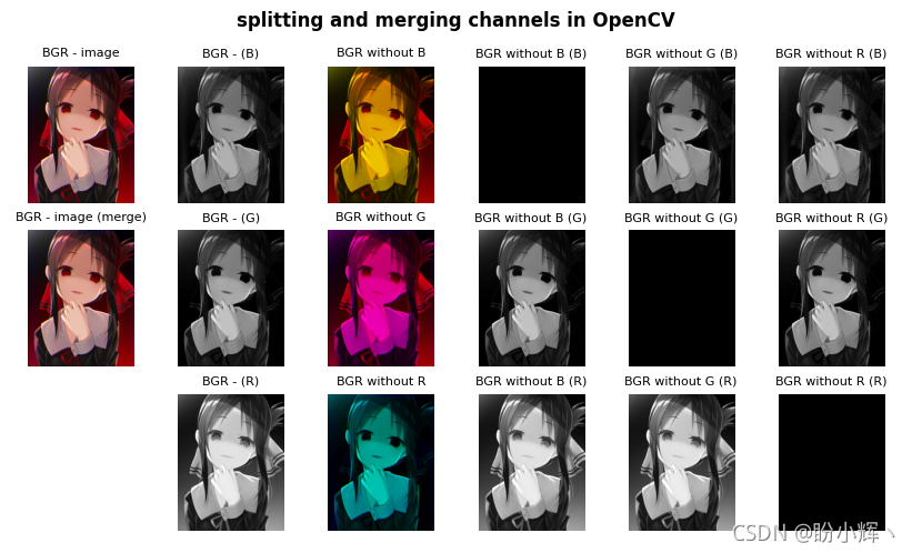
在上图中，也可以更好的看出 RGB 颜色空间的加法属性。例如，没有 B 通道的子图大部分是黄色的，这是因为 绿色+红色 会得到黄色值。

2. 图像的几何变换

几何变换主要包括缩放、平移、旋转、仿射变换、透视变换和图像裁剪等。执行这些几何变换的两个关键函数是 cv2.warpAffine() 和 cv2.warpPerspective()。
cv2.warpAffine() 函数使用以下 2 x 3 变换矩阵来变换源图像：
d s t ( x , y ) = s r c ( M 11 x + M 12 y + M 13 , M 21 x + M 22 y + M 23 ) dst(x,y)=src(M_{11}x+M_{12}y+M_{13}, M_{21}x+M_{22}y+M_{23}) dst(x,y)=src(M11​x+M12​y+M13​,M21​x+M22​y+M23​)
cv2.warpPerspective() 函数使用以下 3 x 3 变换矩阵变换源图像：
d s t ( x , y ) = s r c ( M 11 x + M 12 y + M 13 M 31 x + M 32 y + M 33 , M 21 x + M 22 y + M 23 M 31 x + M 32 y + M 33 ) dst(x,y)=src(\frac {M_{11}x+M_{12}y+M_{13}} {M_{31}x+M_{32}y+M_{33}}, \frac {M_{21}x+M_{22}y+M_{23}} {M_{31}x+M_{32}y+M_{33}}) dst(x,y)=src(M31​x+M32​y+M33​M11​x+M12​y+M13​​,M31​x+M32​y+M33​M21​x+M22​y+M23​​)
接下来，我们将了解最常见的几何变换技术。

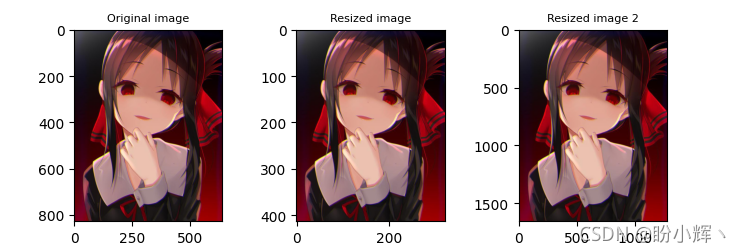
2.1 缩放图像

缩放图像时，可以直接使用缩放后图像尺寸调用 cv2.resize()：

# 指定缩放后图像尺寸
resized_image = cv2.resize(image, (width * 2, height * 2), interpolation=cv2.INTER_LINEAR)

除了上述用法外，也可以同时提供缩放因子 fx 和 fy 值。例如，如果要将图像缩小 2 倍：

# 使用缩放因子
dst_image = cv2.resize(image, None, fx=0.5, fy=0.5, interpolation=cv2.INTER_AREA)

如果要放大图像，最好的方法是使用 cv2.INTER_CUBIC 插值方法(较耗时)或 cv2.INTER_LINEAR。如果要缩小图像，一般的方法是使用 cv2.INTER_LINEAR。
OpenCV 提供的五种插值方法如下表所示：

插值方法	原理
cv2.INTER_NEAREST	最近邻插值
cv2.INTER_LINEAR	双线性插值
cv2.INTER_AREA	使用像素面积关系重采样
cv2.INTER_CUBIC	基于4x4像素邻域的3次插值
cv2.INTER_LANCZOS4	正弦插值

显示缩放后的图像：

def show_with_matplotlib(color_img, title, pos):
    # Convert BGR image to RGB
    img_RGB = color_img[:,:,::-1]
    ax = plt.subplot(1, 3, pos)
    plt.imshow(img_RGB)
    plt.title(title,fontsize=8)
    # plt.axis('off')
show_with_matplotlib(image, 'Original image', 1)
show_with_matplotlib(dst_image, 'Resized image', 2)
show_with_matplotlib(dst_image_2, 'Resized image 2', 3)
plt.show()

可以通过坐标系观察图片的缩放情况：

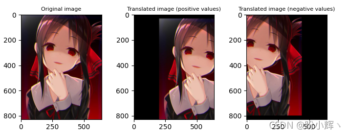
2.2 平移图像

为了平移对象，需要使用 NumPy 数组创建 2 x 3 变换矩阵，其中提供了 x 和 y 方向的平移距离(以像素为单位)：

M = np.float32([[1, 0, x], [0, 1, y]])

其对应于以下变换矩阵：
[ 1 0 t x 0 1 t y ] \begin{bmatrix} 1 & 0 & t_x \\ 0 & 1 & t_y \end{bmatrix} [10​01​tx​ty​​]
创建此矩阵后，调用 cv2.warpAffine() 函数：

dst_image = cv2.warpAffine(image, M, (width, height))

cv2.warpAffine() 函数使用提供的 M 矩阵转换源图像。第三个参数 (width, height) 用于确定输出图像的大小。
例如，如果图片要在 x 方向平移 200 个像素，在 y 方向移动 30 像素：

height, width = image.shape[:2]
M = np.float32([[1, 0, 200], [0, 1, 30]])
dst_image_1 = cv2.warpAffine(image, M, (width, height))

平移也可以为负值，此时为反方向移动：

M = np.float32([[1, 0, -200], [0, 1, -30]])
dst_image_2 = cv2.warpAffine(image, M, (width, height))

显示图片如下：

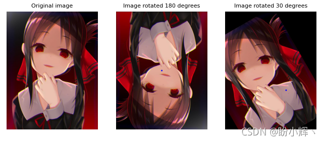
2.3 旋转图像

为了旋转图像，需要首先使用 cv.getRotationMatrix2D() 函数来构建 2 x 3 变换矩阵。该矩阵以所需的角度(以度为单位)旋转图像，其中正值表示逆时针旋转。旋转中心 (center) 和比例因子 (scale) 也可以调整，使用这些元素，以下方式计算变换矩阵：
[ α β ( 1 − a ) ⋅ c e n t e r . x − β ⋅ c e n t e r . y − β α β ⋅ c e n t e r . x − ( 1 − α ) ⋅ c e n t e r . y ] \begin{bmatrix} \alpha & \beta & (1-a)\cdot center.x-\beta\cdot center.y \\ -\beta & \alpha & \beta\cdot center.x-(1-\alpha)\cdot center.y \end{bmatrix} [α−β​βα​(1−a)⋅center.x−β⋅center.yβ⋅center.x−(1−α)⋅center.y​]
其中：
α = s c a l e ⋅ c o s θ , β = s c a l e ⋅ s i n θ \alpha=scale\cdot cos\theta, \beta=scale\cdot sin\theta α=scale⋅cosθ,β=scale⋅sinθ
以下示例构建 M 变换矩阵以相对于图像中心旋转 180 度，缩放因子为 1(不缩放)。之后，将这个 M 矩阵应用于图像，如下所示：

height, width = image.shape[:2]
M = cv2.getRotationMatrix2D((width / 2.0, height / 2.0), 180, 1)
dst_image = cv2.warpAffine(image, M, (width, height))

接下来使用不同的旋转中心进行旋转：

M = cv2.getRotationMatrix2D((width/1.5, height/1.5), 30, 1)
dst_image_2 = cv2.warpAffine(image, M, (width, height))

显示旋转后的图像：

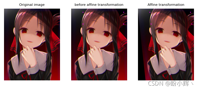
2.4 图像的仿射变换

在仿射变换中，首先需要使用 cv2.getAffineTransform() 函数来构建 2 x 3 变换矩阵，该矩阵将从输入图像和变换图像中的相应坐标中获得。最后，将 M 矩阵传递给 cv2.warpAffine()：

pts_1 = np.float32([[135, 45], [385, 45], [135, 230]])
pts_2 = np.float32([[135, 45], [385, 45], [150, 230]])
M = cv2.getAffineTransform(pts_1, pts_2)
dst_image = cv2.warpAffine(image_points, M, (width, height))

仿射变换是保留点、直线和平面的变换。此外，平行线在此变换后将保持平行。但是，仿射变换不会同时保留像素点之间的距离和角度。
可以通过以下图像观察仿射变换的结果：

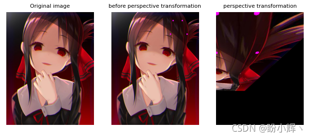
2.5 图像的透视变换

为了进行透视变换，首先需要使用 cv2.getPerspectiveTransform() 函数创建 3 x 3 变换矩阵。该函数需要四对点(源图像和输出图像中四边形的坐标)，函数会根据这些点计算透视变换矩阵。然后，将 M 矩阵传递给 cv2.warpPerspective() ：

pts_1 = np.float32([[450, 65], [517, 65], [431, 164], [552, 164]])
pts_2 = np.float32([[0, 0], [300, 0], [0, 300], [300, 300]])
M = cv2.getPerspectiveTransform(pts_1, pts_2)
dst_image = cv2.warpPerspective(image, M, (300, 300)

透视变换效果如下所示：

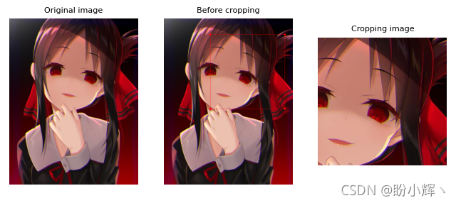
2.6 裁剪图像

可以使用 NumPy 切片裁剪图像：

dst_image = image[80:200, 230:330]

裁剪结果如下所示：

3. 图像滤波

在本节中，将介绍如何模糊和锐化图像，然后应用自定义核。此外，还将介绍一些用于执行其他图像处理功能的常见核。

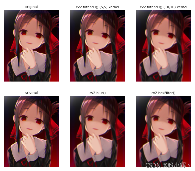
3.1 应用滤波器（卷积核或简称为核）

OpenCV 提供了 cv2.filter2D() 函数，以将任意核应用于图像，将图像与提供的核进行卷积操作。为了使用此函数，首先需要构建将使用的核：

# 使用 5 x 5 核
kernel_averaging_5_5 = np.array([[0.04, 0.04, 0.04, 0.04, 0.04], [0.04,
0.04, 0.04, 0.04, 0.04], [0.04, 0.04, 0.04, 0.04, 0.04],[0.04, 0.04, 0.04,
0.04, 0.04], [0.04, 0.04, 0.04, 0.04, 0.04]])

以上示例创建了 5 x 5 平均卷积核，也可以使用以下方式创建卷积核核：

kernel_averaging_5_5 = np.ones((5, 5), np.float32) / 25

然后将应用 cv2.filter2D() 函数将核应用于源图像：

smooth_image_f2D = cv2.filter2D(image, -1, kernel_averaging_5_5)

上述方法可以将任意核应用于图像。示例中，创建了一个平均卷积核来平滑图像。或者，我们也可以使用 OpenCV 内置的函数，从而在无需创建核的情况下执行图像平滑(也称为图像模糊)。

3.2 图像平滑

平滑技术通常用于减少噪声，此外，这些技术还可用于减少低分辨率图像中的像素化。

3.2.1 均值滤波

可以使用 cv2.blur() 或 cv2.boxFilter() 通过将图像与核卷积来执行均值滤波，在使用 cv2.boxFilter() 时可以不执行规范化，只是取核区域下所有像素的平均值，并用这个平均值替换中心元素，可以控制核大小和锚点位置(默认情况下锚点位于核中心)。当 cv2.boxFilter() 的 normalize 参数等于 True 时，两个函数完全等价。两个函数都使用如下核平滑图像：
K = α [ 1 1 ⋯ 1 1 1 ⋯ 1 ⋮ ⋮ ⋱ ⋮ 1 1 ⋯ 1 ] K=\alpha\begin{bmatrix} 1 & 1 & \cdots & 1 \\ 1 & 1 & \cdots & 1\\ \vdots&\vdots&\ddots&\vdots \\ 1 & 1 & \cdots & 1 \end{bmatrix} K=α⎣⎢⎢⎢⎡​11⋮1​11⋮1​⋯⋯⋱⋯​11⋮1​⎦⎥⎥⎥⎤​
cv2.boxFilter() 函数：
α = { k s i z e . w i d t h ⋅ k s i z e . h e i g h t , if normalize=true 1 , otherwise \alpha = \begin{cases} ksize.width\cdot ksize.height, & \text{if normalize=true} \\[2ex] 1, & \text{otherwise} \end{cases} α=⎩⎨⎧​ksize.width⋅ksize.height,1,​if normalize=trueotherwise​
在 cv2.blur() 函数的情况下：
α = k s i z e . w i d t h ⋅ k s i z e . h e i g h t \alpha = ksize.width\cdot ksize.height α=ksize.width⋅ksize.height
换句话说， cv2.blur() 是使用归一化的 boxFilter()：

# 以下两行代码是等价的
smooth_image_b = cv2.blur(image, (10, 10))
smooth_image_bfi = cv2.boxFilter(image, -1, (10, 10), normalize=True)

均值滤波后的图像如下所示：

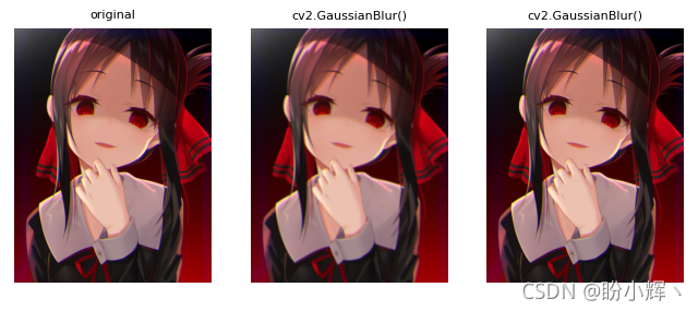
3.2.2 高斯滤波

OpenCV 提供了 cv2.GaussianBlur() 函数用于高斯滤波，该函数使用高斯核对图像进行模糊处理。可以使用以下参数控制高斯核：ksize (核大小)、sigmaX (高斯核 x 方向的标准差) 和 sigmaY (高斯核 y 方向的标准差)。为了获取所应用的高斯核，可以使用 cv2.getGaussianKernel() 函数构建高斯核：

# (9, 9)表示高斯矩阵的长与宽都是5，标准差取0
smooth_image_gb = cv2.GaussianBlur(image, (9, 9), 0)
# 标准差取0.3
smooth_image_gb_2 = cv2.GaussianBlur(image, (9, 9), 0.3)
# 构建高斯核
print(cv2.getGaussianKernel(9,0))

高斯滤波后的图像如下所示：

3.2.3 中值滤波

OpenCV 提供了 cv2.medianBlur() 函数用于中值滤波，该函数使用中值核对图像进行模糊处理：

smooth_image_mb = cv2.medianBlur(image, 9)
smooth_image_mb_2 = cv2.medianBlur(image, 3)

此滤波器可用于减少图像中的椒盐噪声，效果如下：

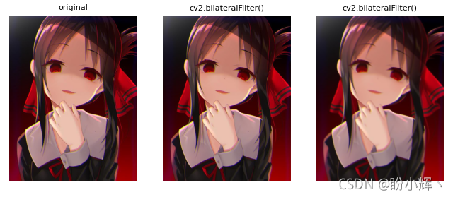
3.2.4 双边滤波

cv2.bilateralFilter() 函数应用于输入图像可以执行双边滤波。与上述所有平滑滤波器倾向于全局平滑不同，此函数可用于在保持边缘锐利的同时减少噪声：

smooth_image_bf = cv2.bilateralFilter(image, 5, 10, 10)

双边滤波效果如下图所示：

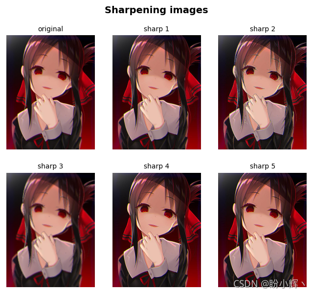
3.3 图像锐化

锐化图像的边缘的一种简单方法是执行非锐化蒙版 (unsharp masking)，即从原始图像中减去图像的非锐化或平滑版本。在以下示例中，首先应用了高斯平滑滤波器，然后从原始图像中减去生成的图像：

smoothed = cv2.GaussianBlur(img, (9, 9), 10)
unsharped = cv2.addWeighted(img, 1.5, smoothed, -0.5, 0)

另一种方法是使用特定的核来锐化边缘，然后应用 cv2.filter2D() 函数：

kernel_sharpen_1 = np.array([[0, -1, 0],
                             [-1, 5, -1],
                             [0, -1, 0]])

kernel_sharpen_2 = np.array([[-1, -1, -1],
                             [-1, 9, -1],
                             [-1, -1, -1]])

kernel_sharpen_3 = np.array([[1, 1, 1],
                             [1, -7, 1],
                             [1, 1, 1]])

kernel_sharpen_4 = np.array([[-1, -1, -1, -1, -1],
                             [-1, 2, 2, 2, -1],
                             [-1, 2, 8, 2, -1],
                             [-1, 2, 2, 2, -1],
                             [-1, -1, -1, -1, -1]]) / 8.0

sharp_image_1 = cv2.filter2D(image, -1, kernel_sharpen_1)
sharp_image_2 = cv2.filter2D(image, -1, kernel_sharpen_2)
sharp_image_3 = cv2.filter2D(image, -1, kernel_sharpen_3)
sharp_image_4 = cv2.filter2D(image, -1, kernel_sharpen_4)

锐化后图像输出如下所示：

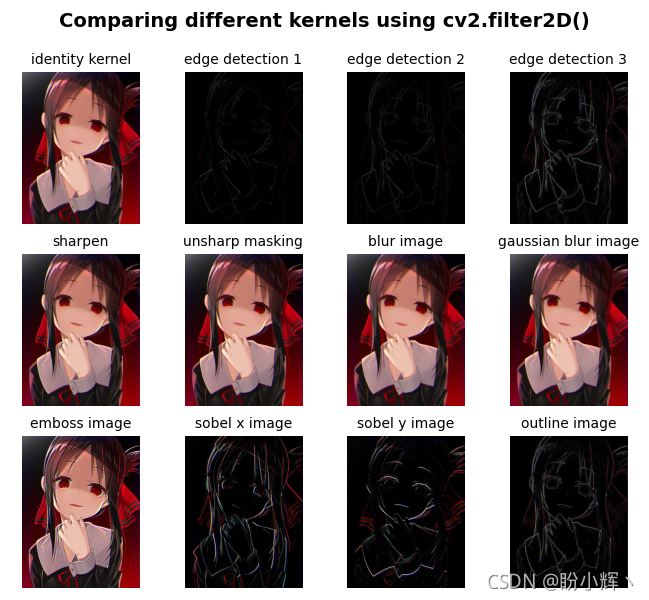
3.4 图像处理中的常用滤波器

还可以定义了一些用于不同目的的通用核，例如：边缘检测、平滑、锐化或浮雕等，定义内核后，可以使用 cv2.filter2D() 函数：

image = cv2.imread('sigonghuiye.jpeg')

kernel_identity = np.array([[0, 0, 0], 
                            [0, 1, 0], 
                            [0, 0, 0]])

# 边缘检测
kernel_edge_detection_1 = np.array([[1, 0, -1],
                                    [0, 0, 0],
                                    [-1, 0, 1]])

kernel_edge_detection_2 = np.array([[0, 1, 0],
                                    [1, -4, 1],
                                    [0, 1, 0]])

kernel_edge_detection_3 = np.array([[-1, -1, -1],
                                    [-1, 8, -1],
                                    [-1, -1, -1]])

# 锐化
kernel_sharpen = np.array([[0, -1, 0],
                           [-1, 5, -1],
                           [0, -1, 0]])

kernel_unsharp_masking = -1 / 256 * np.array([[1, 4, 6, 4, 1],
                                              [4, 16, 24, 16, 4],
                                              [6, 24, -476, 24, 6],
                                              [4, 16, 24, 16, 4],
                                              [1, 4, 6, 4, 1]])

# 模糊
kernel_blur = 1 / 9 * np.array([[1, 1, 1],
                                [1, 1, 1],
                                [1, 1, 1]])

gaussian_blur = 1 / 16 * np.array([[1, 2, 1],
                                   [2, 4, 2],
                                   [1, 2, 1]])

# 浮雕
kernel_emboss = np.array([[-2, -1, 0],
                          [-1, 1, 1],
                          [0, 1, 2]])

# 边缘检测
sobel_x_kernel = np.array([[1, 0, -1],
                           [2, 0, -2],
                           [1, 0, -1]])

sobel_y_kernel = np.array([[1, 2, 1],
                           [0, 0, 0],
                           [-1, -2, -1]])

outline_kernel = np.array([[-1, -1, -1],
                           [-1, 8, -1],
                           [-1, -1, -1]])

# 应用卷积核
original_image = cv2.filter2D(image, -1, kernel_identity)
edge_image_1 = cv2.filter2D(image, -1, kernel_edge_detection_1)
edge_image_2 = cv2.filter2D(image, -1, kernel_edge_detection_2)
edge_image_3 = cv2.filter2D(image, -1, kernel_edge_detection_3)
sharpen_image = cv2.filter2D(image, -1, kernel_sharpen)
unsharp_masking_image = cv2.filter2D(image, -1, kernel_unsharp_masking)
blur_image = cv2.filter2D(image, -1, kernel_blur)
gaussian_blur_image = cv2.filter2D(image, -1, gaussian_blur)
emboss_image = cv2.filter2D(image, -1, kernel_emboss)
sobel_x_image = cv2.filter2D(image, -1, sobel_x_kernel)
sobel_y_image = cv2.filter2D(image, -1, sobel_y_kernel)
outline_image = cv2.filter2D(image, -1, outline_kernel)

总结

在本文中，介绍了计算机视觉项目中常见的图像处理技术，主要包括图像的几何变换和图像滤波等。

相关链接

OpenCV-Python实战（1）——OpenCV简介与图像处理基础（内含大量示例，📕建议收藏📕）
OpenCV-Python实战（2）——图像与视频文件的处理（两万字详解，️📕建议收藏📕）
OpenCV-Python实战（3）——OpenCV中绘制图形与文本（万字总结，️📕建议收藏📕）