牛顿法(Newton's Method)
前言正文代码实现迭代可视化
前言
牛顿法 (Newton’s Method) 是一种迭代优化算法,用于求解无约束优化问题中的局部最小值。它通过使用目标函数的二阶导数信息来逼近最优解,并在每次迭代中更新当前估计的最优解。以下是关于牛顿法的详细描述:
初始化参数:选择一个初始点 x ( 0 ) x^{(0)} x(0) 作为优化的起始点。选优过程: 对于每次迭代 t t t :计算目标函数 f ( x ( t ) ) f\left(x^{(t)}\right) f(x(t)) 在当前点 x ( t ) x^{(t)} x(t) 处的梯度 ∇ f ( x ( t ) ) \nabla f\left(x^{(t)}\right) ∇f(x(t)) 和 Hessian 矩阵 ∇ 2 f ( x ( t ) ) \nabla^2 f\left(x^{(t)}\right) ∇2f(x(t)) 。解牛顿方程 ∇ 2 f ( x ( t ) ) δ x ( t ) = − ∇ f ( x ( t ) ) \nabla^2 f\left(x^{(t)}\right) \delta x^{(t)}=-\nabla f\left(x^{(t)}\right) ∇2f(x(t))δx(t)=−∇f(x(t)) ,其中 δ x ( t ) \delta x^{(t)} δx(t) 是更新的步长。更新参数: x ( t + 1 ) = x ( t ) + δ x ( t ) x^{(t+1)}=x^{(t)}+\delta x^{(t)} x(t+1)=x(t)+δx(t) 。 停止条件: 检查是否满足停止条件。可能的停止条件包括: 达到预定的迭代次数。梯度的范数小于某个容许误差。更新的参数变化小于某个容许误差。 输出结果:输出最终的参数 x ( t ) x^{(t)} x(t) ,以及在最优点的目标函数值 f ( x ( t ) ) f\left(x^{(t)}\right) f(x(t)) 。牛顿法相较于梯度下降法的优点在于:
快速收敛:在一些情况下,牛顿法能够更快地收敛到最优解。充分利用二阶奮息:通过使用目标函数的二阶导数信息,提供了更多关于函数形状的信息。然而,牛顿法也有一些缺点:
计算开销大:计算和存储 Hessian 矩阵可能很昂贵,尤其在高维问题中。可能陷入局部最小值: 由于牛顿法是一个局部优化方法,初始点的选择可能导致陷入局部最小值。为了解决一些计算开销大的问题,有一些变种的牛顿法,如拟牛顿法 (Quasi-Newton Methods),其中不需要显式计算 Hessian 矩阵。
正文
使用牛顿法计算目标函数 f ( x ) = x ( 1 ) 2 + x ( 2 ) 2 − 2 x ( 1 ) x ( 2 ) + sin ( x ( 1 ) ) + f(x)=x(1)^2+x(2)^2-2 x(1) x(2)+\sin (x(1))+ f(x)=x(1)2+x(2)2−2x(1)x(2)+sin(x(1))+ cos ( x ( 2 ) ) \cos (x(2)) cos(x(2)) 的过程如下:
初始化参数:选择一个初始点 x ( 0 ) x^{(0)} x(0) 作为优化的起始点。选代过程: 对于每次迭代 t t t :计算目标函数在当前点 x ( t ) x^{(t)} x(t) 处的梯度和 Hessian 矩阵。∇ f ( x ( t ) ) = [ 2 x 1 − 2 x 2 + cos ( x 1 ) 2 x 2 − 2 x 1 − sin ( x 2 ) ] ∇ 2 f ( x ( t ) ) = [ 2 − sin ( x 1 ) − 2 − 2 2 − cos ( x 2 ) ] \begin{aligned} & \nabla f\left(x^{(t)}\right)=\left[\begin{array}{cc} 2 x_1-2 x_2+\cos \left(x_1\right) \\ 2 x_2-2 x_1-\sin \left(x_2\right) \end{array}\right] \\ & \nabla^2 f\left(x^{(t)}\right)=\left[\begin{array}{cc} 2-\sin \left(x_1\right) & -2 \\ -2 & 2-\cos \left(x_2\right) \end{array}\right] \end{aligned} ∇f(x(t))=[2x1−2x2+cos(x1)2x2−2x1−sin(x2)]∇2f(x(t))=[2−sin(x1)−2−22−cos(x2)]解牛顿方程 ∇ 2 f ( x ( t ) ) δ x ( t ) = − ∇ f ( x ( t ) ) \nabla^2 f\left(x^{(t)}\right) \delta x^{(t)}=-\nabla f\left(x^{(t)}\right) ∇2f(x(t))δx(t)=−∇f(x(t)) ,得到更新的步长 δ x ( t ) \delta x^{(t)} δx(t) 。
[ 2 − sin ( x 1 ) − 2 − 2 2 − cos ( x 2 ) ] [ δ x 1 ( t ) δ x 2 ( t ) ] = − [ 2 x 1 − 2 x 2 + cos ( x 1 ) 2 x 2 − 2 x 1 − sin ( x 2 ) ] \left[\begin{array}{cc} 2-\sin \left(x_1\right) & -2 \\ -2 & 2-\cos \left(x_2\right) \end{array}\right]\left[\begin{array}{l} \delta x_1^{(t)} \\ \delta x_2^{(t)} \end{array}\right]=-\left[\begin{array}{l} 2 x_1-2 x_2+\cos \left(x_1\right) \\ 2 x_2-2 x_1-\sin \left(x_2\right) \end{array}\right] [2−sin(x1)−2−22−cos(x2)][δx1(t)δx2(t)]=−[2x1−2x2+cos(x1)2x2−2x1−sin(x2)]更新参数: x ( t + 1 ) = x ( t ) + δ x ( t ) x^{(t+1)}=x^{(t)}+\delta x^{(t)} x(t+1)=x(t)+δx(t) 。 停止条件:检查是否满足停止条件。可能的停止条件包括: 达到预定的迭代次数。
・梯度的范数小于某个容许误差。更新的参数变化小于某个容许误差。 輸出结果: 输出最终的参数 x ( t ) x^{(t)} x(t) ,以及在最优点的目标函数值 f ( x ( t ) ) f\left(x^{(t)}\right) f(x(t)) 。
这个过程中的关键步骤是计算梯度和 Hessian 矩阵,然后解牛顿方程以获得更新的步长。牛顿法使用了目标函数的二阶信息,因此在一些情况下,它可能更快地收敛到最优解。但需要注意,牛顿法的计算开销可能很大,尤其是在高维问题中。
代码实现
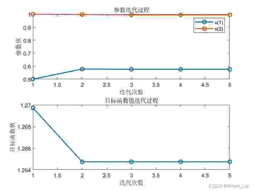
% 定义目标函数f = @(x) x(1)^2 + x(2)^2 - 2*x(1)*x(2) + sin(x(1)) + cos(x(2));% 定义目标函数的梯度grad_f = @(x) [2*x(1) - 2*x(2) + cos(x(1)); 2*x(2) - 2*x(1) - sin(x(2))];% 定义目标函数的 Hessian 矩阵hessian_f = @(x) [2 - sin(x(1)), -2; -2, 2 - cos(x(2))];% 设置参数max_iterations = 1000;tolerance = 1e-6;% 初始化起始点x = [0; 0];% 存储迭代过程中的参数和目标函数值history_x = zeros(2, max_iterations);history_f = zeros(1, max_iterations);% 牛顿法迭代for iteration = 1:max_iterations % 计算梯度和 Hessian 矩阵 gradient = grad_f(x); hessian = hessian_f(x); % 解牛顿方程并更新参数 delta_x = -inv(hessian) * gradient; x = x + delta_x; % 存储迭代过程中的参数和目标函数值 history_x(:, iteration) = x; history_f(iteration) = f(x); % 检查停止条件 if norm(gradient) < tolerance break; endend% 可视化迭代过程figure;subplot(2, 1, 1);plot(1:iteration, history_x(1, 1:iteration), '-o', 'LineWidth', 1.5);hold on;plot(1:iteration, history_x(2, 1:iteration), '-o', 'LineWidth', 1.5);title('参数迭代过程');legend('x(1)', 'x(2)');xlabel('迭代次数');ylabel('参数值');subplot(2, 1, 2);plot(1:iteration, history_f(1:iteration), '-o', 'LineWidth', 1.5);title('目标函数值迭代过程');xlabel('迭代次数');ylabel('目标函数值');% 显示最终结果fprintf('最优解: x = [%f, %f]\n', x(1), x(2));fprintf('f(x)的最优值: %f\n', f(x));fprintf('迭代次数: %d\n', iteration);迭代可视化