需要源码和数据集请点赞关注收藏后评论区留言私信~~~

下面对天池项目中的红酒数据集进行分析与挖掘

实现步骤

1：导入模块

2：颜色和打印精度设置

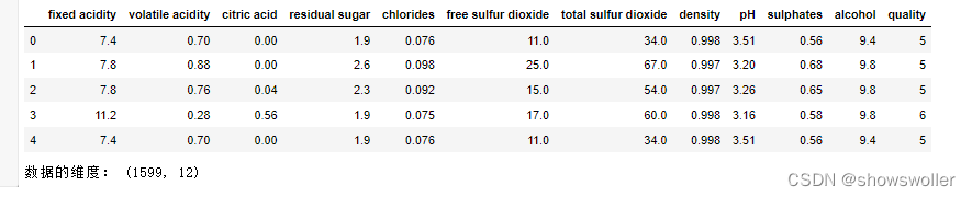
3：获取数据并显示数据维度

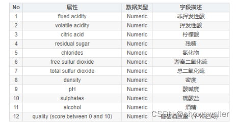
字段中英文对照表如下

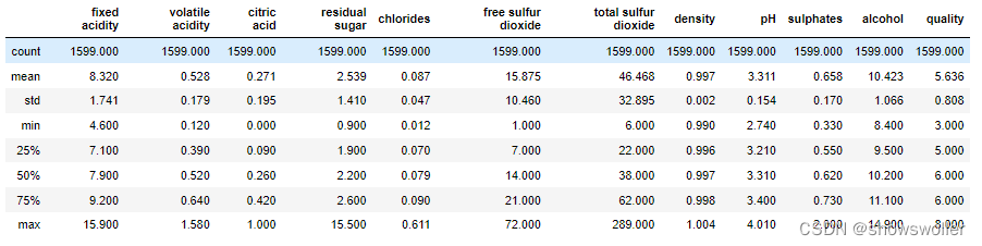
然后利用describe函数显示数值属性的统计描述值

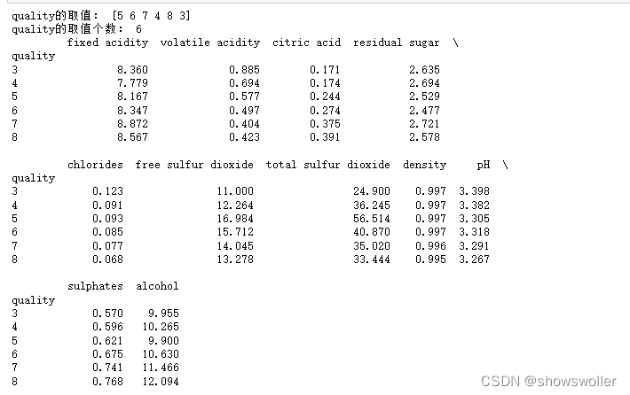
 显示quality取值的相关信息

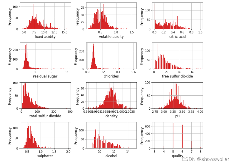
显示各个变量的直方图如下

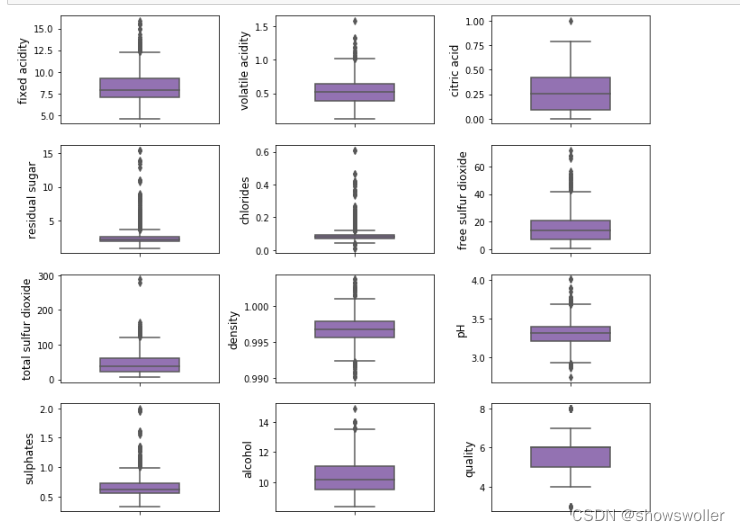
 显示各个变量的盒图

酸性相关的特征分析 该数据集与酸度相关的特征有’fixed acidity’, ‘volatile acidity’, ‘citric acid’,‘chlorides’, ‘free sulfur dioxide’, ‘total sulfur dioxide’,‘PH’。其中前6中酸度特征都会对PH产生影响。PH在对数尺度，然后对6中酸度取对数做直方图

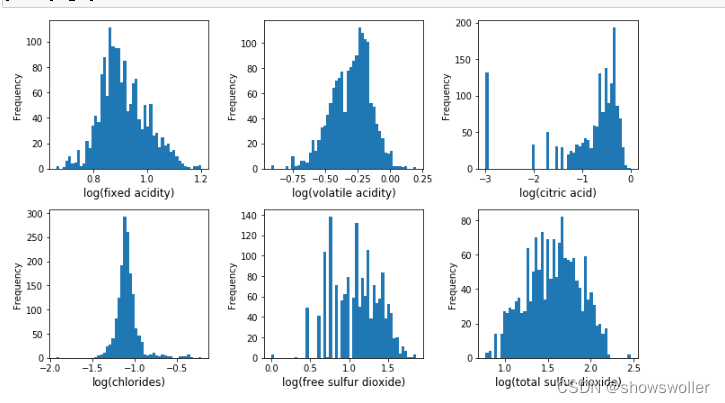
pH值主要是与fixed acidity有关，fixed acidity比volatile acidity和citric acid高1到2个数量级(Figure 4)，比free sulfur dioxide, total sulfur dioxide, sulphates高3个数量级。   一个新特征total acid来自于前三个特征的和

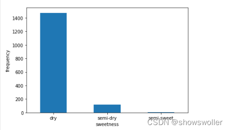
 甜度（sweetness） residual sugar主要与酒的甜度有关，干红（<= 4g/L），半干（4-12g/L），半甜（12-45g/L），甜（>= 45g/L），该数据集中没有甜葡萄酒

绘制甜度的直方图如下

 绘制不同品质红酒的各个属性的盒图

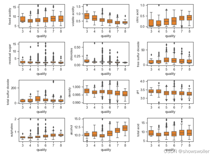
从上图可以看出：

红酒品质与柠檬酸，硫酸盐，酒精度成正相关 红酒品质与易挥发性酸，密度，PH成负相关 残留糖分，氯离子，二氧化硫对红酒品质没有什么影响

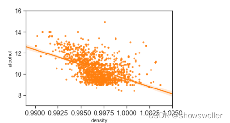
下面分析密度和酒精浓度的关系

密度和酒精浓度是相关的，物理上，但两者并不是线性关系。另外密度还与酒精中的其中物质含量有关，但是相关性很小

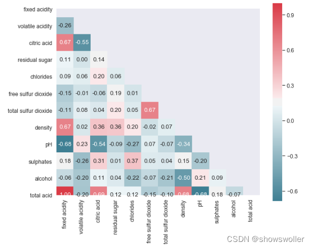
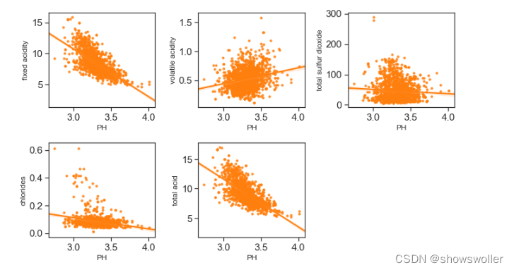
 酸性物质含量和PH 因为PH和非挥发性酸之间存在着-0.68的相关性，因为非挥发性酸的总量特别高，所以total acid这个指标意义不大

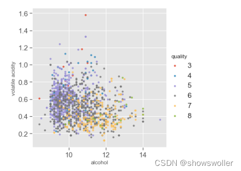
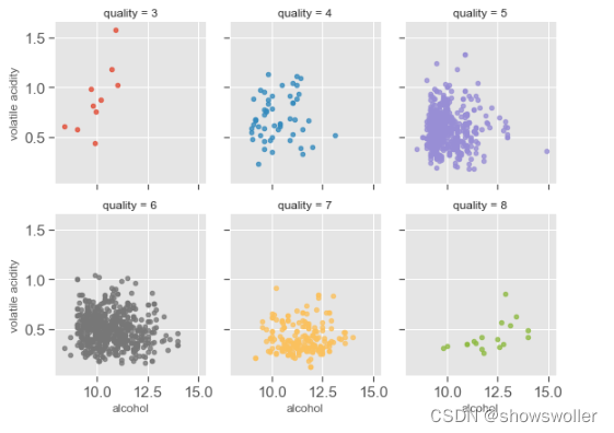
多变量分析 与红酒品质相关性最高的三个特征分别是酒精浓度，挥发性酸含量，柠檬酸。下面研究三个特征对红酒的品质有何影响

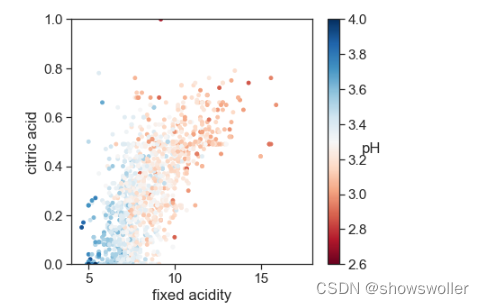
PH和非挥发性酸，柠檬酸成负相关

总结 对于红酒品质影响最重要的三个特征：酒精度、挥发性酸含量和柠檬酸。对于品质高于7的优质红酒和品质低于4的劣质红酒，直观上线性可分，对于品质为5和6的红酒很难进行线性区分

 随机森林、线性回归等算法部分

对数据类型编码，将数据集划分为训练集和测试集等等

对比原始数据与做了标准化处理的数据，其结果相差不大，所以该数据集不需要做标准化处理

下面我们展示各种算法的预测精度结果

可以发现误差都比较大，其中随机森林误差较高

 代码

部分代码如下 需要全部代码请点赞关注收藏后评论区留言私信~~~

#!/usr/bin/env python# coding: utf-8# ## 数据分析部分# In[1]:import numpy as npimport pandas as pdimport matplotlib.pyplot as pltimport seaborn as sns# from sklearn.datasets import load_wine# In[2]:# 颜色color = sns.color_palette()# 数据print精度pd.set_option('precision',3) # In[3]:df = pd.read_csv('.\winequality-red.csv',sep = ';')display(df.head())print('数据的维度：',df.shape)# ![image.png](attachment:image.png)# In[4]:df.info()# In[5]:df.describe()# In[6]:print('quality的取值：',df['quality'].unique())print('quality的取值个数：',df['quality'].nunique())print(df.groupby('quality').mean())# 显示各个变量的直方图# In[ ]:# In[7]:color = sns.color_palette()column= df.columns.tolist()fig = plt.figure(figsize = (10,8))for i in range(12):    plt.subplot(4,3,i+1)    df[column[i]].hist(bins = 100,color = color[3])    plt.xlabel(column[i],fontsize = 12)    plt.ylabel('Frequency',fontsize = 12)plt.tight_layout()# 显示各个变量的盒图# In[8]:fig = plt.figure(figsize = (10,8))for i in range(12):    plt.subplot(4,3,i+1)    sns.boxplot(df[column[i]],orient = 'v',width = 0.5,color = color[4])    plt.ylabel(column[i],fontsize = 12)plt.tight_layout()# 酸性相关的特征分析# 该数据集与酸度相关的特征有’fixed acidity’, ‘volatile acidity’, ‘citric acid’,‘chlorides’, ‘free sulfur dioxide’, ‘total sulfur dioxide’,‘PH’。其中前6中酸度特征都会对PH产生影响。PH在对数尺度，然后对6中酸度取对数做直方图。# In[9]:acidityfeat = ['fixed acidity', 'volatile acidity', 'citric acid', 'chlorides', 'free sulfur dioxide', 'total sulfur dioxide',]fig = plt.figure(figsize = (10,6))for i in range(6):    plt.subplot(2,3,i+1)    v = np.log10(np.clip(df[acidityfeat[i]].values,a_min = 0.001,a_max = None))    plt.hist(v,bins = 50,color = color[0])    plt.xlabel('log('+ acidityfeat[i] +')',fontsize = 12)    plt.ylabel('Frequency')    plt.tight_layout()# In[10]:plt.figure(figsize=(6,3))bins = 10**(np.linspace(-2,2)) # linspace 默认50等分plt.hist(df['fixed acidity'], bins=bins, edgecolor = 'k', label='Fixed Acidity') #bins: 直方图的柱数，可选项，默认为10plt.hist(df['volatile acidity'], bins=bins, edgecolor = 'k', label='Volatitle Acidity')#label:字符串或任何可以用'%s'转换打印的内容。plt.hist(df['citric acid'], bins=bins, edgecolor = 'k', label='Citric Acid')plt.xscale('log')plt.xlabel('Acid Concentration(g/dm^3)')plt.ylabel('Frequency')plt.title('Histogram of Acid Contacts')#title ：图形标题plt.legend()#plt.legend（）函数主要的作用就是给图加上图例plt.tight_layout()print('Figure 4')"""pH值主要是与fixed acidity有关，fixed acidity比volatile acidity和citric acid高1到2个数量级(Figure 4)，比free sulfur dioxide, total sulfur dioxide, sulphates高3个数量级。   一个新特征total acid来自于前三个特征的和。"""# 甜度（sweetness）# residual sugar主要与酒的甜度有关，干红（<= 4g/L），半干（4-12g/L），半甜（12-45g/L），甜（>= 45g/L），该数据集中没有甜葡萄酒。# In[11]:df['sweetness'] = pd.cut(df['residual sugar'],bins = [0,4,12,45],labels = ['dry','semi-dry','semi-sweet'])df.head()# In[12]:plt.figure(figsize = (6,4))df['sweetness'].value_counts().plot(kind = 'bar',color = color[0])plt.xticks(rotation = 0)plt.xlabel('sweetness')plt.ylabel('frequency')plt.tight_layout()print('Figure 5')# In[13]:# 创建一个新特征total aciddf['total acid'] = df['fixed acidity'] + df['volatile acidity'] + df['citric acid']columns = df.columns.tolist()columns.remove('sweetness')# columns# ['fixed acidity',#  'volatile acidity',#  'citric acid',#  'residual sugar',#  'chlorides',#  'free sulfur dioxide',#  'total sulfur dioxide',#  'density',#  'pH',#  'sulphates',#  'alcohol',#  'quality',#  'total acid']sns.set_style('ticks')sns.set_context('notebook',font_scale = 1.1)column = columns[0:11] + ['total acid']plt.figure(figsize = (10,8))for i in range(12):    plt.subplot(4,3,i+1)    sns.boxplot(x = 'quality',y = column[i], data = df,color = color[1],width = 0.6)    plt.ylabel(column[i],fontsize = 12)plt.tight_layout()print('Figure 7:PhysicoChemico Propertise and Wine Quality by Boxplot')# 从上图可以看出：# # 红酒品质与柠檬酸，硫酸盐，酒精度成正相关# 红酒品质与易挥发性酸，密度，PH成负相关# 残留糖分，氯离子，二氧化硫对红酒品质没有什么影响# In[14]:sns.set_style('dark')plt.figure(figsize = (10,8))mcorr = df[column].corr()mask = np.zeros_like(mcorr,dtype = np.bool)mask[np.triu_indices_from(mask)] = Truecmap = sns.diverging_palette(220, 10, as_cmap=True)g = sns.heatmap(mcorr, mask=mask, cmap=cmap, square=True, annot=True, fmt='0.2f')# print('Figure 8:Pairwise colleration plot')# In[ ]:# In[15]:# 密度和酒精浓度# 密度和酒精浓度是相关的，物理上，但两者并不是线性关系。另外密度还与酒精中的其中物质含量有关，但是相关性很小。sns.set_style('ticks')sns.set_context('notebook',font_scale = 1.4)plt.figure(figsize = (6,4))sns.regplot(x = 'density',y = 'alcohol',data = df,scatter_kws = {'s':10},color = color[1])plt.xlabel('density',fontsize = 12)plt.ylabel('alcohol',fontsize = 12)plt.xlim(0.989,1.005)plt.ylim(7,16)# print('Figure 9: Density vs Alcohol')# 酸性物质含量和PH# 因为PH和非挥发性酸之间存在着-0.68的相关性，因为非挥发性酸的总量特别高，所以total acid这个指标意义不大。# In[16]:column# In[17]:acidity_raleted = ['fixed acidity','volatile acidity','total sulfur dioxide','chlorides','total acid']plt.figure(figsize = (10,6))for i in range(5):    plt.subplot(2,3,i+1)    sns.regpltx = 'pH',y = acidity_raleted[i],data = df,scatter_kws = {'s':10},color = color[1])    plt.xlabel('PH',fontsize = 12)    plt.ylabel(acidity_raleted[i],fontsize = 12)    plt.tight_layout()print('Figure 10:The correlation between different acid and PH')# 多变量分析# 与红酒品质相性最高的三个特征分别是酒精浓度，挥发性酸含量，柠檬酸。下面研究三个特征对红酒的品质有何影响。# In[18]:plt.style.use('ggplot')plt.figure(figsize = (6,4))sns.lmplot(x = 'alcohol',y = 'volatile acidity',hue = 'quality',data = df,fit_reg = False,scatter_kws = {'s':10},size = 5)# In[19]:sns.lmplot(x = 'alcohol', y = 'volatile acidity', col='quality', hue = 'quality',            data = df,fit_reg = False, size = 3,  aspect = 0.9, col_wrap=3,           ={'s':20})print("Figure 11-2: Scatter Plots of Alcohol, Volatile Acid and Quality")# PH和非挥发性酸，柠檬酸# PH和非挥发性酸，柠檬酸成负相关# In[20]:sns.set_style('ticks')sns.set_context("notebook", font_scale= 1.4)plt.figure(figsize=(6,5))cm = plt.cm.get_cmap('RdBu')sc = plt.scatter(df['fixed acidity'], df['citric acid'], c=df['pH'], vmin=2.6, vmax=4, s=15, cmap=cm)bar = plt.colorbar(sc)bar.n = 0)plt.xlabel('fixed acidity')plt.ylabel('ciric acid')plt.xlim(4,18)plt.ylim(0,1)print('Figure 12: pH with Fixed Acidity and Citric Acid')# 总结# 对于红酒品质影响最重要的三个特征：酒精度、挥发性酸含量和柠檬酸。对于品质高于7的优质红酒和品质低于4的劣质红酒，直观上线性可分，对于品质为5和6的红酒很难进行线性区分。# ## 数据掘时间部分# In[21]:# 数据建模# 线性回归# 集成算法# 提升算# 模型评估# 确定模型参数# 1.数据集切分# 1.1 切分特征和标签# 1.2 切分训练集个测试集df.head()# In[22]:# 数据预处理工作# 检查数据的完整性df.isnull().sum()# In[23]:# 将object类型的数据转化为int类型sweetness = pd.get_dummies(df['sweetness'])df = pd.concat([df,sweetness],axis = 1)df.head()# In[24]:df = df.drop('sweetness',axis = 1)labels = df['quality']features = df.drop('quality',axis = 1)# 对原始数据集进行切分from sklearn.model_selection import train_test_splittrain_features,test_fatures,train_labels,test_labels = train_test_split(features,labels,test_size = 0.3,random_state = 0print('训练特征的规模:'.shape)print('训练标签的规模:',train_labels.shape)print('测试特征的规模:',test_features.shape)print('测试标签的规模:',test_labels.shape)# In[25]:from sklearn import svmclassifier=svm.SVC(kernel='linear',gamma=0.1)classifier.fit(train_features,train_labels)print('训练集的准确率',classifier.score(train_features,train_labels))print('测试集的准确率',classifier.score(test_features,test_labels))# In[26]:from sklearn.linear_model import LinearRegressionLR = LinearRegression)LR.fit(train_features,train_labelsprediction = LR.predict(test_features)prediction[:5]# In[27]:#对模型进行评估from sklearn.metrics import mean_squared_errorRMSE = np.sqrt(mean_squared_error(test_labels,prediction))print('线性回归模型的预测误差:',RMSE)# In[28]:# 对训练特征和测试特征做标准化处理，观察结果from sklearn.preprocessing import StandardScalertrain_features_std = StandardScaler().fit_transform(train_features)test_features_std = StandardScaler().fit_transform(test_features)LR = LinearRegression()LR.fit(train_features_std,train_labels)prediction = LR.predict(test_features_std)#观察预测结果误差RMSE = np.sqrt(mean_squared_error(prediction,test_labels))print('线性回归模型预测误差:',RMSE)# 对比原始数据与做了标准化处理的数据，其结果相差不大，所以该数据集不需要做标准化处理。# # 集成算法：随机森林# In[29]:from sklearn.ensemble import RandomForestRegressorRF = RandomForestRegressor()RF.fit(train_features,train_labels)prediction = RF.pre# In[30]:RF.get_params# In[31]:from sklearn.model_selection import GridSearchCVparam_grid = {'n_estimators':[100,200,300,400,500],             'max_depth':[3,4,5,6],             'min_samples_split':[2,3,4]}RF = RandomForestRegressor()grid = GridSearchCV(RF,param_grid = param_grid,scoring = 'neg_mean_squared_error',cv = 3,n_jobs = -1)grid.fit(train_features,train_labels)# In[32]:# GridSearchCV(cv=3, error_score='raise-deprecating',#        estimator=RandomForestRegressor(bootstrap=True, criterion='mse', max_depth=None,#            max_features='auto', max_leaf_nodes=None,#            min_impurity_decrease=0.0, min_impurity_split=None,#            min_samples_leaf=1, min_samples_split=2,#            min_weight_fraction_leaf=0.0, n_estimators='warn', n_jobs=None,#            oob_sc# In[33]:grid.best_params_# In[34]:RF = RandomForestRegressor(n_estimators = 300,min_samples_split = 2,max_depth = 6)RF.fit(train_features,train_labels)# In[35]:RandomForestRe# In[36]:prediction = RF.predict(test_features)RF_RMSE = np.sqrt(mean_squared_error(prediction,test_labels))print('随机森林模型的预测误差:',RF_RMSE)# 集成算法：GBDT# In[37]:from sklearn.ensemble import GradientBoostingRegressorGBDT = GradientBoostingRegressor()GBDT.fit(train_features,train_labels)gbdt_prediction =GBDT.get_params# In[ ]:

创作不易 觉得有帮助请点赞关注收藏~~~