方法介绍
1.Theil-Sen Median方法又被称为 Sen 斜率估计,是一种稳健的非参数统计的趋势计算方法。该方法计算效率高,对于测量误差和离群数据不敏感,常被用于长时间序列数据的趋势分析中。对于后续代码计算结果中的slope.tif解读,当slope大于0表示随时间序列呈现上升趋势;slope小于0表示随时间序列呈现下降趋势。
2.Mann-Kendall是一种非参数统计检验方法,最初由Mann在1945年提出,后由Kendall和Sneyers进一步完善,其优点是不需要测量值服从正态分布,也不要求趋势是线性的,并且不受缺失值和异常值的影响,在长时间序列数据的趋势显著检验中得到了十分广泛的应用。对于后续代码计算结果中的z.tif,当|Z|大于1.65、1.96和2.58时,表示趋势分别通过了置信度为90%、95%和99%的显著性检验。
代码介绍
此代码大部分来自Github大佬分享,我修改了报错的个别代码后亲自测试pycharm下只需改路径就可以运行:
# coding:utf-8'''已全部实现'''import numpy as npimport pymannkendall as mkimport osimport rasterio as rasdef sen_mk_test(image_path, outputPath): # image_path:影像的存储路径 # outputPath:结果输出路径 global path1 filepaths = [] for file in os.listdir(path1): filepath1 = os.path.join(path1, file) filepaths.append(filepath1) # 获取影像数量 num_images = len(filepaths) # 读取影像数据 img1 = ras.open(filepaths[0]) # 获取影像的投影,高度和宽度 transform1 = img1.transform height1 = img1.height width1 = img1.width array1 = img1.read() img1.close() # 读取所有影像 for path1 in filepaths[1:]: if path1[-3:] == 'tif': print(path1) img2 = ras.open(path1) array2 = img2.read() array1 = np.vstack((array1, array2)) img2.close() nums, width, height = array1.shape # 写影像 def writeImage(image_save_path, height1, width1, para_array, bandDes, transform1): with ras.open( image_save_path, 'w', driver='GTiff', height=height1, width=width1, count=1, dtype=para_array.dtype, crs='+proj=latlong', transform=transform1, ) as dst: dst.write_band(1, para_array) dst.set_band_description(1, bandDes) del dst # 输出矩阵,无值区用-9999填充 slope_array = np.full([width, height], -9999.0000) z_array = np.full([width, height], -9999.0000) Trend_array = np.full([width, height], -9999.0000) Tau_array = np.full([width, height], -9999.0000) s_array = np.full([width, height], -9999.0000) p_array = np.full([width, height], -9999.0000) # 只有有值的区域才进行mk检验 c1 = np.isnan(array1) sum_array1 = np.sum(c1, axis=0) nan_positions = np.where(sum_array1 == num_images) positions = np.where(sum_array1 != num_images) # 输出总像元数量 print("all the pixel counts are {0}".format(len(positions[0]))) # mk test for i in range(len(positions[0])): print(i) x = positions[0][i] y = positions[1][i] mk_list1 = array1[:, x, y] trend, h, p, z, Tau, s, var_s, slope, intercept = mk.original_test(mk_list1) ''' trend: tells the trend (increasing, decreasing or no trend) h: True (if trend is present) or False (if trend is absence) p: p-value of the significance test z: normalized test statistics Tau: Kendall Tau s: Mann-Kendal's score var_s: Variance S slope: Theil-Sen estimator/slope intercept: intercept of Kendall-Theil Robust Line ''' if trend == "decreasing": trend_value = -1 elif trend == "increasing": trend_value = 1 else: trend_value = 0 slope_array[x, y] = slope # senslope s_array[x, y] = s z_array[x, y] = z Trend_array[x, y] = trend_value p_array[x, y] = p Tau_array[x, y] = Tau all_array = [slope_array, Trend_array, p_array, s_array, Tau_array, z_array] slope_save_path = os.path.join(result_path, "slope.tif") Trend_save_path = os.path.join(result_path, "Trend.tif") p_save_path = os.path.join(result_path, "p.tif") s_save_path = os.path.join(result_path, "s.tif") tau_save_path = os.path.join(result_path, "tau.tif") z_save_path = os.path.join(result_path, "z.tif") image_save_paths = [slope_save_path, Trend_save_path, p_save_path, s_save_path, tau_save_path, z_save_path] band_Des = ['slope', 'trend', 'p_value', 'score', 'tau', 'z_value'] for i in range(len(all_array)): writeImage(image_save_paths[i], height1, width1, all_array[i], band_Des[i], transform1)# 调用path1 = r"E:\Test\ACMEI\ACMEI"result_path = r"E:\Test\ACMEI\ACMEImk"sen_mk_test(path1, result_path)后续处理三步走
1.对于生成的tif栅格,只需要取slope.tif以及z.tif进行重分类。
slope>0赋值1表示增加 |z|>1.96赋值2表示显著
slope=0赋值0表示不变 |z|<=1.96赋值1表示不显著
slope<0赋值-1表示减少
(此处还可根据显著性阈值再细分为更多类,我仅作基本演示分为5类)
2.再相乘得到
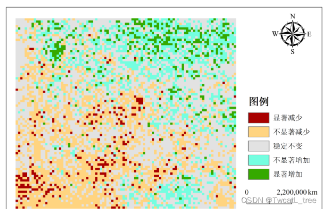
-2:显著减少;-1:不显著减少;0:稳定不变;1:不显著增加; 2:显著增加
3.在Arcmap出图即可!